Extras: Type 2 Systems Examples

Let's say that we have a unity-feedback system as shown below

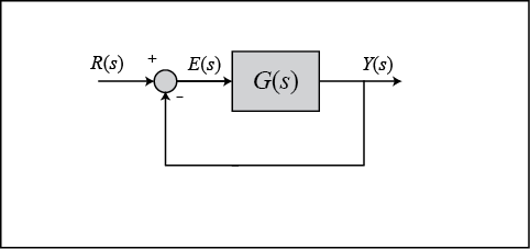
where G(s) is the following.

(1) $\frac{(s+1)(s+3)}{s^2(s+2)(s+3)}$

Note that we are using a different numerator in our transfer function than we used for the type 0 and type 1 systems in order to make sure we have a stable closed-loop system.

Let's look at the closed-loop response for this system when we use different inputs.

Step Input

s = tf('s');
G = ((s+1)*(s+3))/(s^2*(s+2)*(s+3));
sys_cl = feedback(G,1);
[y,t] = step(sys_cl);
u = ones(size(t));
plot(t,y,'b',t,u,'g')
axis([0,48,0,2])
xlabel('Time(secs)')
ylabel('Amplitude')
title('Input-green, Output-blue')

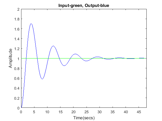
Our steady-state error is zero.

Ramp Input

s = tf('s');
G = ((s+1)*(s+3))/(s^2*(s+2)*(s+3));
sys_cl = feedback(G,1);
t = 0:0.1:50;
u = t;
[y,t,x] = lsim(sys_cl,u,t);
plot(t,y,'b',t,u,'g')
xlabel('Time(secs)')
ylabel('Amplitude')
title('Input-green, Output-blue')

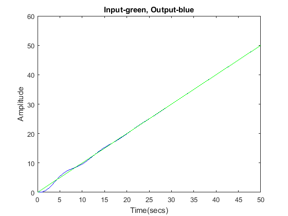
Our steady-state error is zero.

Parabolic Input

s = tf('s');
G = ((s+1)*(s+3))/(s^2*(s+2)*(s+3));
sys_cl = feedback(G,1);
t = 0:0.1:20;
u = 0.5*t.*t;
[y,x] = lsim(sys_cl,u,t);
plot(t,y,'b',t,u,'g')
xlabel('Time(secs)')
ylabel('Amplitude')
title('Input-green, Output-blue')
%

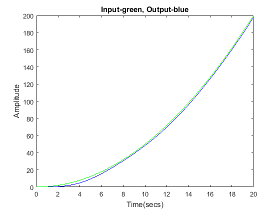
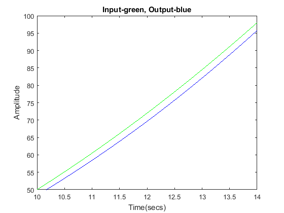
Our steady-state error is constant, but it's kind of hard to see. Therefore, we will zoom in to examine this steady-state error.

axis([10,14,50,100])
xlabel('Time(secs)')
ylabel('Amplitude')
title('Input-green, Output-blue')