Activity 4: Temperature Control of a Lightbulb

Key Topics: Blackbox Modeling, First-Order Systems, ON/OFF Control, PI Control, Steady-state Error, Embedded Control

Equipment needed
Purpose
System identification experiment
ON/OFF Control
P and PI Control
Embedded Control

Equipment needed

Arduino board (e.g. Uno, Mega 2560, etc.)
lightbulb (incandescent, LED, CFL, etc.)
AC solid-state relay (hockey-puck type, etc.)
temperature sensor (TMP36, etc.)

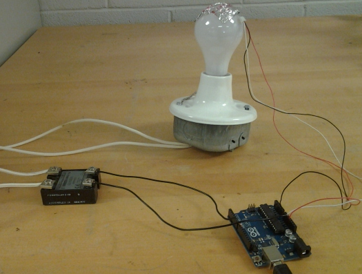
The temperature of the lightbulb is measured in this example with a TMP36 sensor (cheap, relatively accurate, sufficient range). The Arduino board provides power to the sensor and reads the sensor output via an Analog Input. The Arduino board is also used for generating the Digital Output that switches the solid-state relay on and off. That is, the digital output alternately connects and disconnects the light bulb from the AC power source (from the wall) via the relay in order to turn the light bulb on and off. The control logic employed for determining when to switch the relay on and off is implemented within Simulink, which is also employed for visualizing the lightbulb's temperature and the control signal.

Purpose

The purpose of this activity with the lightbulb is to demonstrate how to control switched systems. The lightbulb's temperature is increased by turning the lightbulb on and the lightbulb's temperature is decreased by turning the lightbulb off (up to environmental limits). The lightbulb is a binary system with only two states, on or off. The lightbulb is either connected to the AC source or it is not; its intensity cannot be modulated. In this experiment, we observe the resulting "chattering" behavior of the lightbulb and investigate alternative methodologies for reducing the frequency of this chatter, or smoothing the chatter, through the use of deadbands, low-pass filters, and Pulse-Width Modulation. This activity also provides exposure to Proportional (P) control, Proportional-Integral (PI) control, and first-order systems.

System identification experiment

In order to implement our temperature control system, we technically don't need a model of our plant (the lightbulb). We can simply employ logic that turns the lightbulb on when the measured temperature is lower than desired and turns the lightbulb off when the temperature is higher than desired. We, however, would like to be able to explain the resulting behavior of our control system (and perhaps even attempt to design the control algorithm in a more intelligent manner). Therefore, we will generate a model for the thermal behavior of the lightbulb based on its observed response. This is sometimes referred to as a blackbox model or a data-driven model. After we have generated such a model, we will attempt to explain what we have observed based on our understanding of the underlying physics.

Hardware setup

In this experiment our plant is a standard incandescent lightbulb where we will (ultimately) attempt to control the lightbulb's temperature. We have chosen a 25 W bulb in order to keep the maximum temperature within the limits of the temperature sensor we have chosen. You can also employ other types of bulbs (LED, CFL, etc.).

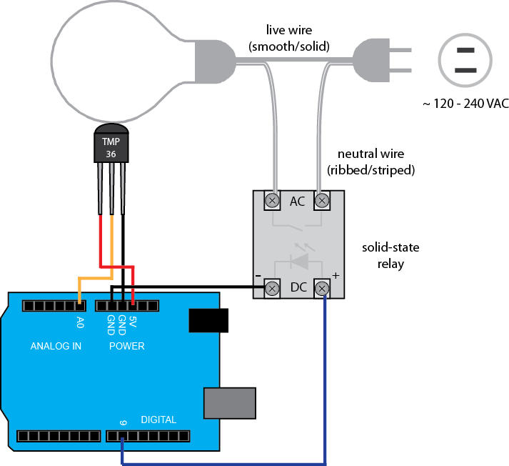
For our temperature sensor, we will employ the TMP36 (though many others can be employed). This sensor measures temperature in Celsius, is quite inexpensive (a couple of dollars), has adequate range, reasonable accuracy, and doesn't need to be calibrated. This sensor is also commonly included in many Arduino starter kits that are in the market place. The datasheet for this sensor can be found here. The temperature sensor can be attached to the surface of the lightbulb employing thermally conductive epoxy, or with adhesive metal tape. The TMP36 is connected to the Arduino Board as shown below. Specifically, if the sensor is oriented such that the pins are pointed downward and the flat side of the sensor is facing you, then the leftmost pin is the power (must be between 2.7 V and 5.5 V), the middle pin is the signal, and the rightmost pin is ground. Power and ground for the TMP36 are supplied from the Arduino board and the signal, which is a voltage that is linearly proportional to temperature, is read on one of the board's Analog Inputs.

The lightbulb is turned on and off employing a digital output from the Arduino board via a solid-state relay. The solid-state relay is basically an electrical switch that can connect/disconnect a (possibly high-power) device to an AC source with a low-power DC signal. In our case, the AC source comes from a standard wall outlet and the DC signal is supplied by a Digital Output from our Arduino board. Therefore, our solid-state relay needs to be able to handle 120-240 V on the AC side (in North America need 120 V) and the DC side must be able to be controlled with a 5 V signal. Since our load (the lightbulb) is resistive (not inductive) and doesn't require much current, we don't have to be very particular about the solid-state relay we employ. We are in particular employing a simple "hockey-puck" style relay. In order to control the lightbulb, we need to insert the relay into the circuit (the loop) that connects the lightbulb to the wall. Therefore, we must cut into the cord for the lightbulb and wire the relay into the circuit. In doing this, make sure that the bulb is not plugged in. You should insert the relay on the neutral wire of the bulb's plug. The neutral wire is indicated by a white stripe or ribbing. If you insert the relay on the live wire, then the terminals of the relay are connected to the power supply even when the relay is off. You should also cover the exposed terminals of the relay and never touch the terminals when the bulb is plugged in.

Software setup

In this experiment, we will employ Simulink to command the relay, to read the data from the temperature sensor, and to plot the data in real time. In particular, we will employ the IO package from the MathWorks. For details on how to use the IO package, refer to the following link. Later on, we demonstrate how to embed the control logic on-board the Arduino board.

The Simulink model we will use is shown below and can be downloaded here, where you may need to change the COM port in the IO Setup block to match location where your Arduino board is connected. This model reads the temperature data via an Analog Read on channel A0. This data is then converted from counts to degrees Celsius. The raw temperature data is expressed in numbers of bits. The Arduino Board employs a 10-bit analog-to-digital converter. This means (for the default) an Analog Input channel reads a voltage between 0 and 5 V and slices that range into $2^{10} = 1024$ pieces. Therefore, an output of 0 corresponds to 0 V and an output of 1023 corresponds to 5 V. Since the maximum output voltage from the TMP36 is 1.75 V, you can get better resolution by employing the on-board 3.3 V source for AREF instead of using the default 5 V. The data in bits is then converted to millivolts (assuming the default 5 V reference) before being converted to temperature in degrees Celsius. This last conversion is based on information given in the datasheet for the TMP36. The model then displays the stored data on a scope and a display and is written to the MATLAB workspace for further analysis.

This model commands the relay to be open (1) or closed (0) (corresponding to the lightbulb on and off, respectively) via a Digital Write on channel 9. For starters, we will employ a step input such that the lightbulb is initially off and is turned on once. The Arduino Analog Read block, Digital Write block, IO Setup block, and Real-Time Pacer block are all part of the IO package. The remaining blocks are part of standard Simulink libraries, specifically, they can be found under the Math, Sinks, and Sources libraries.

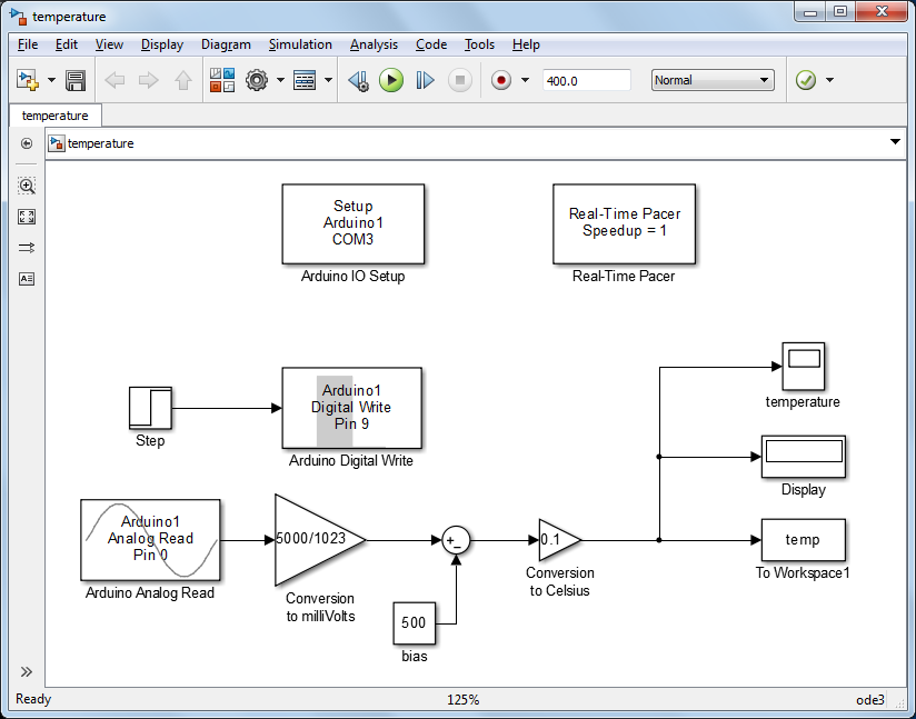
Double-clicking on the Analog Read block, we can change the "Sample time." The fastest that the system can be sampled, while allowing real-time communication and plotting with Simulink, is about once every 0.01 seconds. If you try to sample too quickly, the Simulink model will run slower than real-time, that is, it won't be able to sample at the rate specified. Since the thermal dynamics of the lightbulb are relatively slow, a sample time of 0.1 is more than sufficient. We will set the sample time within the Digital Write block to the same value.

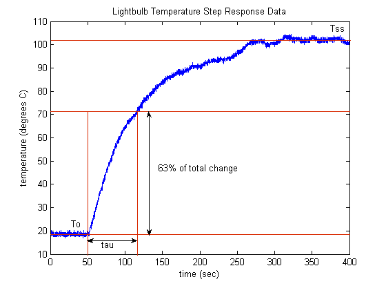
Once the Simulink model has been created, it can then be run to collect a set of data like that shown below. Specifically, the lightbulb is initially at ambient temperature when the model is started. At time t = 50 seconds the lightbulb is turned on (via the step input) and it is allowed to heat up. We wait 50 seconds before turning the lightbulb on in order to gather sufficient data for estimating the ambient temperature (initial lightbulb temperature). Make sure to run the model for a sufficient amount of the time for the lightbulb temperature to reach steady state.

Inspection of the above response data indicates that the thermal dynamics of the lightbulb appear to be approximately first order. We will employ this fact to derive a model for the lightbulb.

Modeling

In this experiment, we will derive a model for the thermal dynamics of the lightbulb solely based on the step response data we recorded. That is, we will fit a model to the data without any consideration of the underlying physics of the system. Examination of the recorded data indicates that the thermal dynamics of the lightbulb are approximately first order. Therefore, we will fit a transfer function to the data of the form shown below, where $K$ is the system's DC gain and $\tau$ is the system's time constant.

(1) $P(s) = \frac{Y(s)}{U(s)} = \frac{K}{\tau s + 1}$

For our particular lightbulb system, we will consider the input to be the percent of time the lightbulb is on (i.e. duty cycle), $D(s)$ , and we will consider the output to be the deviation of the light bulb's temperature $T$ from the ambient temperature $T_o$ , $\Delta T(s)$ . We chose our output to be $\Delta T$ rather than simply $T$ in order to give us a linear model. Recalling the definition of a linear system, the output must be linearly proportional to the input. This means that an input of 0 must generate an output of 0.

Examining the recorded data above, there are some challenges in estimating the parameters $K$ and $\tau$ because of the noise on the signal and because of the drift in the data. The effect of the noise could be minimized by low-pass filtering, or smoothing, the data. We will in essence do this in our heads by just "eye-balling" an average curve fitted to the data. The drift could be due to a variety of external effects, for example, variations in the ambient temperature, gusts of air (convection), variation in the amplitude of the voltage, errors in the sensor, etc. We again will try to average over this variation by considering an approximate average of the data.

From inspection of the given step response data, the ambient temperature (initial lightbulb temperature) appears to be approximately 18.5 degrees C, while the steady-state lightbulb temperature appears to be about 102 degrees C. Since the input is equal to 1 (100 percent duty cycle), and the output is $\Delta T$ , this means the DC gain $K$ of the system is approximately 83.5 degrees C (102 - 18.5). Recalling the definition of time constant as the time it takes for the system response to achieve 63% of its total change, the time constant for this system appears to be approximately 66 seconds. See below for an annotated version of the step response plot where 0.63(83.5 degrees) + 18.5 degrees is approximately 71.1 degrees, which occurs at approximately 116 seconds. Since the step input didn't occur until 50 seconds, that means the time constant is approximately 66 seconds (116 - 50).

Based on the above identification of parameters, the estimated model of the lightbulb's thermal dynamics is then the following.

(2) $P(s) = \frac{\Delta T(s)}{D(s)} = \frac{83.5}{66s + 1}\ ^{\circ}C$

In order to get a better sense of how well our derived model fits our data, we will apply the following MATLAB commands, where the output of our Simulink model from above, temp, is saved as a timeseries.

         s = tf('s');
         To = 18.5;            % ambient/initial temperature
         K = 83.5;             % DC gain
         tau = 66;             % time constant
         P = K/(tau*s+1);      % model transfer function
         [y,t] = step(P,350);  % model step response
         plot(t+50,y+To);
         hold
         plot(temp,'r:')
         xlabel('time (sec)')
         ylabel('temperature (degrees C)')
         title('Lightbulb Temperature Step Response')
         legend('model','experiment','Location','SouthEast')

Examination of the above demonstrates that our assumption of a first-order model seems to be a reasonable one. This shouldn't surprise us too much if we consider the underlying physics of the lightbulb. Considering the heat balance for the lightbulb, we have the following:

Considering the rate of energy storage depends on the "thermal capacitance" of the light bulb, while the net rate of heat transfer depends on the thermal conductivity of the light bulb (like the inverse of "thermal resistance") and the difference between the bulb's temperature and the temperature of the environment, and the heat generation is the system's input (will be almost a perfect step because the electrical dynamics are so fast), we have the following governing equation for the system.

(3) $C \frac{dT}{dt} = -\frac{1}{R}(T - T_o) + u$

Rewriting the above in terms of $\Delta T = T - T_o$ , we can make use of the fact that $T_o$ is approximately constant, that is $\dot{\Delta T} = \dot{T}$ , which leads to the following.

(4) $RC \dot{\Delta T} + \Delta T = u$

Inspection of the above shows that the thermal dynamics of the lightbulb are modeled by a first-order differential equation whose dynamics are the same as an RC circuit with time constant $\tau = RC$ .

ON/OFF Control

Now that we have some intuition about the behavior of our plant and a model, we can attempt some strategies for its control. Specifically, we will attempt to control the temperature of the lightbulb. The first approach to control that we will attempt is a simple ON/OFF controller that turns the lightbulb on when the measured temperature is less than the desired temperature (error > 0) and turns the lightbulb off when the measured temperature is greater than the desired temperature (error < 0). Below shows our modified Simulink model with the logic of our ON/OFF controller implemented using a Switch block with a reference temperature of 75 degrees Celsius. This model can be downloaded here.

The control scheme shown above does not use any knowledge of the plant model and employs feedback. The feedback loop is a little difficult to picture because the plant is in the physical world. The figure below helps to illustrate how the entire feedback system (the Simulink model and the physical world) fits together.

It is instructive to take a minute and think about how you would implement an open-loop controller for this system (no measurement of the lightbulb's temperature) based on our previously derived model. What would be the advantages and disadvantages of such an approach?

The resulting temperature of our lightbulb with the closed-loop ON/OFF controller is shown below. The behavior is pretty intuitive. Initially the lightbulb is too cold causing the controller to turn the bulb on. This causes the bulb to heat up. It takes approximately 75 seconds for the bulb's temperature to first reach the desired temperature of 75 degrees Celsius with the lightbulb fully on. At this point, the light bulb then is turned off because its temperature has risen above the desired level. As the bulb loses heat to the environment, its temperature decreases until it falls below 75 degrees, at which point the lightbulb is turned back on. This ON/OFF control strategy then results in the lightbulb flickering, being rapidly turned on and off, and the resulting temperature chatters around the desired temperature. This flickering can be further exacerbated by noise in the measured temperature signal.

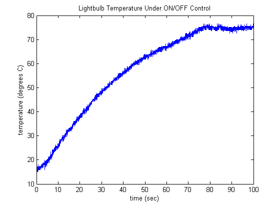
This resulting control is quite effective in that it keeps the lightbulb's temperature close to the desired level and was designed and implemented without a high level of knowledge. A possible drawback of this approach is that it may shorten the life of the lightbulb and it may not be very energy efficient. Such considerations are common to other applications of ON/OFF control. We will now consider a couple of approaches for reducing the chatter observed in the lightbulb's temperature.

With Low-pass Filter

One approach for reducing the chatter is to add a low-pass filter on the temperature measurement. In the model shown below, we employ a simple first-order filter with a time constant equal to 2 seconds. The filter acts on the $\Delta T$ signal to account for the fact that a transfer function assumes zero initial conditions. This model can be downloaded here.

The resulting controlled behavior is shown below. Here we can see the effect of the low pass filter to smooth the measured temperature signal. One way to make sense of this is to consider what a first-order step response looks like. It in essence takes a fast moving signal (a step) and rounds it off, where a larger time constant increases the rounding (decreases the speed of response of the filter). Another way to make sense of the filter is to consider it as a moving average of the current and previous temperature measurements. One can arrive at this interpretation by considering a discrete-time version of the filter transfer function. In this case, a larger time constant puts more weight on the older measurements in the moving average.

This approach to filtering could have been employed when we generated our blackbox model of the plant. One drawback of using a low-pass filter in real time is that it adds lag to the signal as can be seen below.

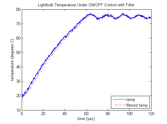
Aside from smoothing the noise in the temperature measurement signal, the filter also reduced the frequency with which the light bulb was turned on and off, thereby possibly improving the life and efficiency of the lightbulb. The drawback is that the controlled temperature does not stay as close to the commanded temperature. These relative effects can be influenced by changing the time constant of the filter. The reason why the filter affects the lightbulb in this manner can be understood by considering the low-pass filter as a moving average. When there is no filter, as soon as the temperature rises above the desired level the lightbulb turns off and as soon as the temperature falls below the desired level the lightbulb turns on. With a moving average, the lightbulb will not turn off when the temperature reaches the threshold because the average has not yet crossed the threshold. The average is weighed down by all of the old (lower) measurements. We have to wait for several of the most recent measurements to cross the threshold in order to counteract the older measurements below the threshold.

With Deadband

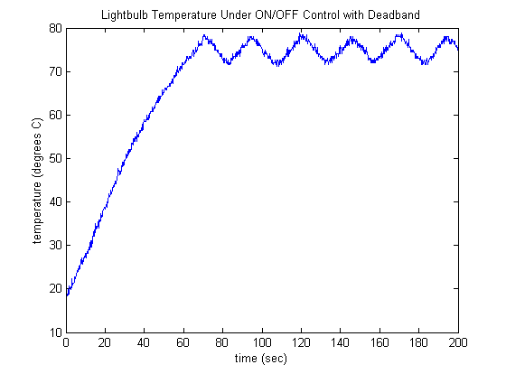
An alternative to employing a low-pass filter to reduce the frequency with which the light bulb turns on and off is to use a deadband. This is achieved in the model shown below with a Relay block. The Relay block behaves like a switch with hysteresis, that is, it has a different condition for switching "ON" than it does for switching "OFF." In this case, the deadband is set to +2/-2 degrees. In other words, the lightbulb is turned off when the measured temperature rises 2 degrees above desired (77 degrees in this case), and it turns on when the temperature falls 2 degrees below desired (73 degrees in this case). The model shown below with deadband can be downloaded here.

The resulting controlled temperature is shown below, where the effective behavior is similar to that achieved with filtering. The frequency with which the light bulb is turned on and off (and the resulting proximity to the desired temperature) can be affected by changing the size of the deadband.

P and PI Control

In our prior attempts to control temperature we employed ON/OFF control where the lightbulb was fully on when the error was positive and fully off when the error was negative. A more sophisticated approach to control would modulate the lightbulb in proportion to how much temperature error there was (and later, in proportion to the integral of the error as well). In other words, if the lightbulb was much too cool (large error), it would be turned on brightly, but if the lightbulb was only a little cool (small error), it would only be turned on dimly. This approach, where the control effort is proportional to the error, is called Proportional Control or P Control. Mathematically, this is expressed as $control = K_P \cdot error$ . This approach to control won't achieve improved performance compared to the ON/OFF strategies employed so far, but the dynamics of this system are slow enough, and understandable enough, that this exercise will help us to better under P and PI control as it applies in other situations.

P Control

In our system, we control the temperature of the lightbulb by alternately connecting and disconnecting it from the AC power source. As such, we cannot modulate the intensity of the lightbulb, it is either connected to the power source or it is not. We can, however, approximate a continuous P control strategy by using what is termed Pulse-Width Modulation (PWM). In Pulse-Width Modulation the input signal is a pulse train (a square wave) with a constant period (frequency) that switches between 1 and 0 (fully on and fully off, as we have here). The "intensity" of the control is then affected by changing the percent of time that the input is "on." This percentage is called the Duty Cycle. A depiction of a PWM signal is shown below.

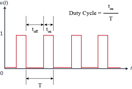
Considering a first-order system, as we have here, you can imagine what the lightbulb's temperature might look like if the period of the PWM signal was very long. You would have a first-order step response rising to some steady-state value (when on), followed by the temperature decaying to ambient (when off). In practice, however, the period of the PWM signal is made small (frequency large) compared to the dynamics of the system being controlled so that there isn't much time for the output to rise or fall. Therefore, modulating the duty cycle of a PWM input can achieve an approximately smoothly changing output.

The model given below implements a P Control strategy for our lightbulb system. The PWM signal is implemented by the Analog Write block shown. This block represents the duty cycle as an 8-bit number ( $2^8 = 256$ ). Therefore, the input to the Analog Write block must be between 0 and 255, where 0 corresponds to a $0\%$ duty cycle and 255 maps to a $100\%$ duty cycle. The saturation block is included to capture these limits. The PWM signal is output on the Digital Pin 9 that we have been utilizing. Those digital pins that can generate a PWM output are indicated by the ~ symbol on the Arduino board. The model shown below can be downloaded here.

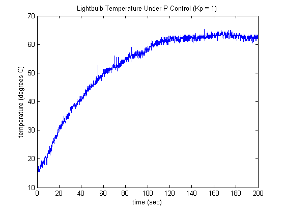
To begin, we will arbitrarily pick a proportional gain of $K_p = 1$ . The resulting temperature profile with this gain is shown below. The resulting profile has a significant amount of steady-state error as compared to the supplied reference temperature of 75 degrees Celsius.

This is to be expected based on the model of the plant we derived earlier, $P(s) = 83.5/(66s + 1)$ , since the resulting control system is type 0. Let's perform some analysis to better understand the behavior we are observing and the effect of the proportional gain in general. An idealized representation of our control system is shown below. Note that the feedback loop is written in terms of $\Delta T$ , rather than $T$ , in order that our plant be linear with zero initial conditions.

For this system with $C(s) = K_p$ and the $P(s)$ defined earlier, we have the following closed-loop transfer function.

(5) $G_{cl}(s) = \frac{C(s)P(s)}{1+C(s)P(s)} = \frac{83.5K_p}{66s + 1 + 83.5K_p}$

Examining the above, we can see that the closed-loop system has a DC gain of $G_{cl}(0) = 83.5K_p/(1 + 83.5K_p)$ . Even with $K_p = 1$ , the DC gain is very close to 1, therefore, the steady-state output of the control system should be closer to the reference of 75 degrees than it is. While it is understandable that the environmental conditions, or the bulb itself, could have changed, such differences don't explain the magnitude of the error observed. The difference between the prediction and the observation is that our model was derived for a step input of 1, that is, for a $100\%$ duty cycle. Looking at the control input generated for $K_p = 1$ shown below, we can see that the lightbulb operates at a duty cycle that is significantly less than $100\%$ .

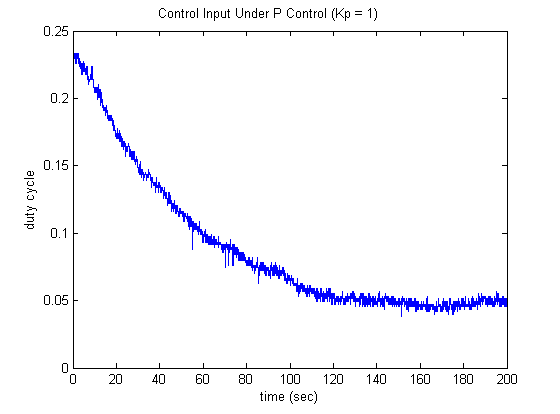
Inspection of the expression for the DC gain that we derived earlier shows that increasing $K_p$ will bring the steady-state gain closer to 1. Also significant is that a larger value of $K_p$ will increase the commanded duty cycle, bringing it closer to the conditions for which our plant model $P(s)$ was derived. Looking at the closed-loop transfer function, we further observe that it is first order with a pole of $-(1+83.5K_p)/66$ . 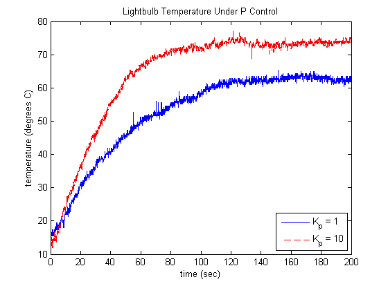Therefore, increasing $K_p$ will still result in a first-order type response, but it will reach steady-state more quickly. Increasing $K_p$ achieves the following temperature profile and requires the following control effort.

An alternative to increasing $K_p$ is to scale the reference $T_{ref}$ so that the steady-state temperature matches the desired. This, however, relies on an accurate and predictable model in order to set the scaling factor correctly. A further alternative is to add integral action to the controller. We will attempt this next.

PI Control

Adding a term to our controller that is proportional to the integral of the error gives us what is termed a Proportional-Integral Controller or a PI Controller for short. Mathematically, this controller has the form $C(s) = K_p + K_i/s$ . Such a controller makes the feedback control system type 1, therefore, it should reduce the steady-state error to a constant reference (a step in essence) to zero. Examining the new closed-loop transfer function shown below, we can investigate this.

(6) $G_{cl}(s) = \frac{C(s)P(s)}{1+C(s)P(s)} = \frac{83.5(K_ps+K_i)}{66s^2 + (1 + 83.5K_p)s + 83.5K_i}$

For this closed-loop transfer function, the DC gain is 1. Therefore, we will indeed have zero steady-state error for a constant reference. The larger the value of $K_i$ , the more quickly the steady-state error will be driven to zero. This behavior makes intuitive sense if we go back to the system's performance we observed with $K_p = 1$ . With that P controller, the lightbulb's temperature reached a steady-state value below the desired. In essence, the control effort (duty-cycle) reached in steady-state supplied energy to the bulb at a rate that was exactly in balance with the rate at which heat was being lost to the environment. The control input remained constant because the temperature error had settled at a steady value and the control effort was proportional to the error. With integral control however, the control effort will continue to increase until it drives the steady-state error to zero. Since integration is a sum, it adds up the area under the error vs. time graph. Therefore, the integral term of the controller will have the effect of increasing the control effort as it accumulates this error (as it adds up the area). A side-effect of the addition of the integral control is that it made our closed-loop system second-order, such that the response may now oscillate (overshoot). This effect is also somewhat intuitive. Let's run our system with a PI controller with $K_p = 1$ and $K_i = 0.02$ and observe the response. Below is a Simulink model with PI control that can be downloaded here.

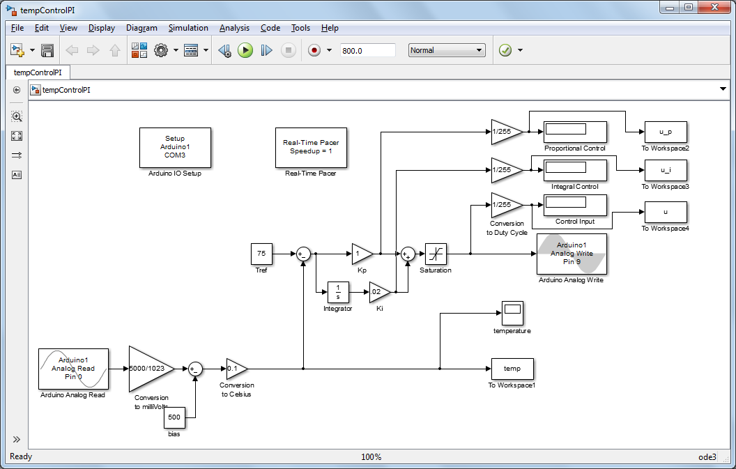
As you run this model, observe the values of the control effort due to the proportional term of the controller and the integral term of the controller (as shown in the displays). Below is given the resulting temperature profile and control effort for this model. Initially the error is large and it gets smaller as the lightbulb heats up. Therefore, the proportional term of the control effort is initially large and then it decreases as the error gets smaller. The integral portion of the control effort continues to grow even as the magnitude of the error decreases because the integral is accumulating error, it is summing the area under the error "curve." When the lightbulb's temperature reaches the desired level, the error is zero and the proportional control effort is also zero. The integral control effort, however, is still quite large because it has accumulated all of the positive error since the control system was started. This is referred to as the integrator "winding up." Therefore, the lightbulb continues to heat up for a while and overshoots its desired temperature due to the integrator. At this point, the error is now negative and the proportional control effort is negative. And while the integral control effort is still positive, it is now starting to decrease. This process of unwinding the integrator takes time. Furthermore, the temperature can then undershoot the desired temperature as it decreases. This example illustrates why our closed-loop system is now second order, that is, why it can now have complex poles and oscillate.

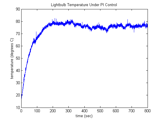
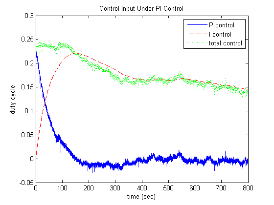
This example also illustrates a common tradeoff with adding integral control. Its addition can help to decrease the steady-state error, but may make the response more oscillatory and slower to settle. Modifying the control gain $K_i$ will alter the balance of these two effects. Returning to our closed-loop transfer function for this feedback system, if we match the denominator to the form of a canonical second order system, $s^2 + 2\zeta\omega_ns + \omega_n^2$ , we see that $83.5K_i = \omega_n^2$ and $1+83.5K_p = 2\zeta\omega_n$ . Therefore, for a constant $K_p$ , increasing $K_i$ increases $\omega_n$ and decreases $\zeta$ , while $\sigma = \zeta\omega_n$ remains constant. This illustrates how increasing $K_i$ can help to drive the error smaller more quickly (decreases rise time due to the larger $\omega_n$ ), but at the cost of more oscillation (increases overshoot due to the smaller $\zeta$ ).

Embedded Control

So far in this experiment, the logic for controlling the lightbulb's temperature has been running in Simulink on a host computer. This was accomplished employing the IO package from the MathWorks which in essence includes a specialized blockset and a program running on board the Arduino for communicating between the board and the host computer running Simulink. The advantage of employing the IO package is that it allows us to communicate with the board in real time with ease. Therefore, we can observe and graph the measured lightbulb temperature (and control effort) during the experiment.

An alternative to running the control logic on the host computer is to instead run the control logic on board the Arduino. This is referred to as "embedding" the control on the microprocessor of the Arduino board. This approach has two advantages. One, since the control software does not have to run under an operating system (i.e. Windows, etc.) that has to address many other (higher priority) tasks, the control program can run faster and achieve faster sampling rates. The other advantage is that Arduino board does not need to be physically connected to the host computer. So for example, if you wanted to create an intelligent stand-alone device to keep your coffee warm, you could do so without needing your device to be plugged into a host computer. Note that if you want to unplug the Arduino board from the host computer, you will then need to provide an alternative power source for the board. For example, the Arduino board can be powered by a 9-V battery plugged into its power jack (7-12 Volts is recommended). In this activity we so far have been powering the board from the host computer through the USB cable.

In order to embed our control logic on board the Arduino, we will use the Arduino Support Package from the MathWorks. More details can be found here. The blockset of this support package is almost identical to those used previously from the IO package. Specifically, the control command (lightbulb on/off) is achieved from a Digital Output block and the temperature is read via an Analog Input block. The Arduino IO Setup block and the Real-Time Pacer block are no longer necessary, though the model needs to be set to automatically detect the COM port, or must be manually set to the correct COM port. This can be done through the drop-down menu of the model toolbar Tools > Run on Target Hardware > Options.... Also the Scope and To Workspace blocks are no longer employed. The implementation of the original ON/OFF controller with Support Package blockset is shown below and can be downloaded here. This control software can be deployed to the Arduino board by clicking on the icon in the upper righthand corner identified by the red circle below, or by typing Ctrl+B. This automatically builds and compiles the Simulink model into code that runs in real time on board the Arduino. This process of Autocode Generation is becoming very common in industrial practice.