


Inverted Pendulum: Frequency Domain Methods for Controller Design
Key MATLAB commands used in this tutorial are: tf , zpkdata , controlSystemDesigner , feedback , impulse
Contents
In this page we will design a controller for the inverted pendulum system using a frequency response design method. In the design process we will assume a single-input, single-output plant as described by the following transfer function. Otherwise stated, we will attempt to control the pendulum's angle without regard for the cart's position.
(1)![$$P_{pend}(s) = \frac{\Phi(s)}{U(s)}=\frac{\frac{ml}{q}s}{s^3+\frac{b(I+ml^2)}{q}s^2-\frac{(M+m)mgl}{q}s-\frac{bmgl}{q}} \qquad [ \frac{rad}{N}]$$](Content/InvertedPendulum/Control/Frequency/html/InvertedPendulum_ControlFrequency_eq14490034572073561881.png)
where,
(2)
The controller we are designing will specifically attempt to maintain the pendulum vertically upward when the cart is subjected to a 1-Nsec impulse. Under these conditions, the design criteria are:
- Settling time of less than 5 seconds
- Pendulum should not move more than 0.05 radians away from the vertical
For the original problem setup and the derivation of the above transfer function, please consult the Inverted Pendulum: System Modeling page.
Note: Applying a frequency response design approach is relatively challenging in the case of this example because the open-loop system is unstable. That is, the open-loop transfer function has a pole in the right-half complex plane. For this reason, attempting this example is not recommended if you are just attempting to learn the basics of applying frequency response techniques. This problem is better suited for more advanced students who wish to learn about some nuances of the frequency response design approach.
System structure
The structure of the controller for this problem is a little different than the standard control problems you may be used to. Since we are attempting to control the pendulum's position, which should return to the vertical after the initial disturbance, the reference signal we are tracking should be zero. This type of situation is often referred to as a regulator problem. The external force applied to the cart can be considered as an impulsive disturbance. The schematic for this problem is depicted below.

You may find it easier to analyze and design for this system if we first rearrange the schematic as follows.

The resulting transfer function  for the closed-loop system from an input of force
  to an output of pendulum angle
  is then determined to be the following.
(3)
Before we begin designing our controller, we first need to define our plant within MATLAB. Create a new m-file and type in the following commands to create the plant model (refer to the main problem for the details of getting these commands).
M = 0.5;
m = 0.2;
b = 0.1;
I = 0.006;
g = 9.8;
l = 0.3;
q = (M+m)*(I+m*l^2)-(m*l)^2;
s = tf('s');
P_pend = (m*l*s/q)/(s^3 + (b*(I + m*l^2))*s^2/q - ((M + m)*m*g*l)*s/q - b*m*g*l/q);
As mentioned above, this system is unstable without control. We can prove this to ourselves by employing the MATLAB command zpkdata. In this case, zpkdata returns the zeros and poles for the transfer function. The added parameter 'v' returns the outputs in the form of vectors instead of cell arrays and can only be employed with single-input, single-output models. Entering the following code in the MATLAB command window generates the output shown below.
[zeros poles] = zpkdata(P_pend,'v')
zeros =
     0
poles =
    5.5651
   -5.6041
   -0.1428
Closed-loop response without compensation
We will now examine the response of the closed-loop system without compensation before we begin to design our controller. In this example, we will employ the Control System Designer for examining the various analysis plots rather than employing individual commands such as bode, nyquist, and impulse. The Control System Designer is an interactive tool with graphical user interface (GUI) which can be launched by the MATLAB command controlSystemDesigner as shown below, or by going to the APPS tab of the MATLAB toolstrip and clicking on the app icon under Control System Design and Analysis.
controlSystemDesigner('bode',P_pend)
The additional parameter 'bode' opens the Control System Designer window with the Bode plot and closed-loop step response of the system  (which was passed to the function) as shown below.

We can then modify the system architecture being employed to reflect the fact that our controller  is in the feedback path of our system as discussed above. This is accomplished from within the Control System Designer window by clicking on the icon labeled Edit Architecture. Then in the new window, modify the default configuration by clicking on the second architecture under Select Control Architecture to match the form shown below.

Next we will begin to examine some of the analysis plots for our system. Recall that we can assess the closed-loop stability
of our system based on the open-loop frequency response. In the case of this example, the open-loop transfer function  of our system is given by the following.
(4)
Note, this is true even though the controller is in the feedback path of the system.
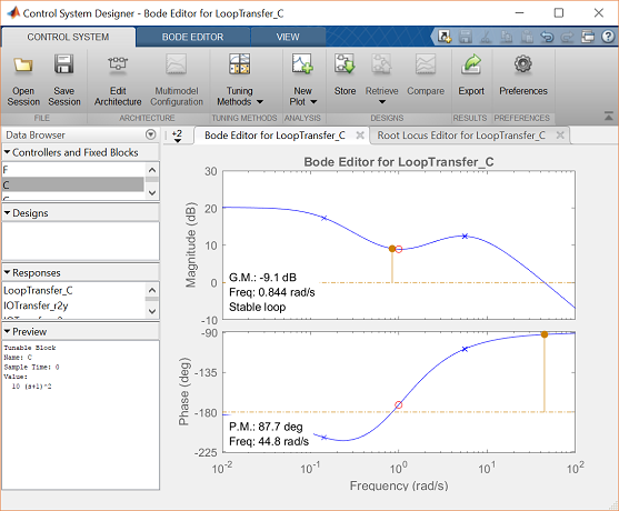
In other examples we have specifically employed a Bode plot representation of the open-loop frequency response. For our system without compensation, we could employ the MATLAB code bode(P_Pend) to generate this Bode plot. Instead, we will use the Control System Designer that we are employing currently. The open-loop Bode plot of our system is already open, but if it weren't, or if we wished to change the type of plot we are employing for design, we could open a new plot from under the New Plot tab of the Control System Designer window as shown below.

Examination of the above Bode plot shows that the magnitude is less than 0 dB and the phase is greater than -180 degrees for all frequencies. For a minimum-phase system this would indicate that the closed-loop system is stable with infinite gain margin and infinite phase margin. However, since our system has a pole in the right-half complex plane, our system is nonminimum phase and the closed-loop system is actually unstable. We will prove this to ourselves by examining a couple of other analysis plots.
In general, when dealing with nonminimum-phase systems it is preferrable to analyze relative stability using the Nyquist plot of the open-loop transfer function. The Nyquist plot is also preferred when analyzing higher-order systems. This is because the Bode plot shows frequencies that are 360 degrees apart as being different when in fact they are the same. Since the Nyquist plot is a polar-type plot, this ambiguity is removed.
In order to generate additional plots to better understand the closed-loop performance of the system, click on the New Plot menu in the toolstrip of the Control System Designer window. The Control System Designer allows the user to view up to eight plots at the same time for analysis. These plots can be viewed for a number of options, such as the open-loop and closed-loop system. We will view the Nyquist plot for the open-loop system and the impulse response of the closed-loop system by following the steps given below.
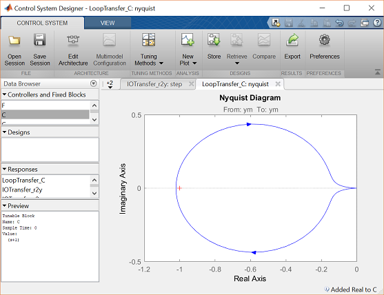
1. Under the New Plot menu, select New Nyquist under Create New Plot. A new window named New Nyquist to plot should appear. In the dropdown menu Select Response to Plot, select New Open-Loop Response. In the boxes Specify the open-loop response at the following locations and Specify the open-loop response with the following loops open, select  . Then click on Plot. You can also select LoopTransfer_C in the dropdown Select Response to Plot to obtain the same Nyquist plot.

2. Under the New Plot menu, select New Impulse under Create New Plot. A new window named New Impulse to plot should appear. In the dropdown menu Select Response to Plot, select IOTransfer_r2y. Then click on Plot.
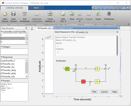
The resulting figure should then appear as follows.

Examination of the above impulse response plot shows that the closed-loop system is unstable. This also can be verified from the open-loop Nyquist plot by applying the Nyquist stability criterion which is stated below.
(5)
Where  is the number of closed-loop poles in the right-half plane,
  is the number of open-loop poles in the right-half plane, and
  is the number of clockwise encirclements of the point -1 by the open-loop Nyquist plot.
From our previous discussion we know that our system has one open-loop pole in the right-half plane ( = 1) and from examination of the open-loop Nyquist plot above we can see that there are no encirclements of the point -1
( = 0). Therefore, = 0 + 1 = 1 and the closed-loop system has 1 pole in the right-half plane indicating that it is indeed unstable.
Closed-loop response with compensation
Since the closed-loop system is unstable without compensation, we need to use our controller to stabilize the system and meet the given requirements. Our first step will be to add an integrator to cancel the zero at the origin. To add an integrator, you may right-click on the Bode plot that is already open and choose Add Pole/Zero > Integrator from the resulting menu. The resulting Bode plot that is generated is shown below and reflects the low frequency behavior we would expect.

If you look at the transfer function closely, you will notice that there is a pole-zero cancellation at the origin. However, the pole-zero cancellation is not automatically recognized by the Control System Designer which can cause numerical errors in the subsequent plots. Therefore, you will need exit out of the Control System Designer tool and re-open the tool with the integrator already added to the plant as shown below.
controlSystemDesigner('bode',minreal(P_pend*(1/s)))
Since the integrator is bundled with the plant which is in the forward path, while our controller is actually in the feedback path, we will not analyze the closed-loop response of this system from within the Control System Designer. However, the open-loop transfer function is unchanged by whether the controller is in the forward or feedback path, therefore, we can still use the plots of the open-loop system for analysis and design. The resulting Bode plot that is generated is shown below.

Even with the addition of this integrator, the closed-loop system is still unstable. We can attempt to better understand the instability (and how to resolve it) by looking more closely at the Nyquist plot. We can generate this analysis plot in the same manner we did previously. Following these steps generates a figure like the one given below.

Notice that the open-loop Nyquist plot now encircles the -1 point in the clockwise direction. This means that the closed-loop
system now has two poles in the right-half plane ( ). Hence, the closed-loop system is still unstable. We need to add phase in order to get a counterclockwise encirclement.
We will do this by adding a zero to our controller. For starters, we will place this zero at -1 and view the resulting plots.
This action can be achieved graphically by right-clicking on the plot as we did previously. Instead, we will add the zero
from the Compensator Editor window of the Control System Designer, which can be opened by right-clicking on the Nyquist plot and then selecting Edit Compensator. Then, right-click in the Dynamics section of the Compensator Editor window and select Add Pole/Zero > Real Zero from the resulting menu. By default, the location of the resulting zero is -1. The resulting window should appear as shown
in the figure below.
). Hence, the closed-loop system is still unstable. We need to add phase in order to get a counterclockwise encirclement.
We will do this by adding a zero to our controller. For starters, we will place this zero at -1 and view the resulting plots.
This action can be achieved graphically by right-clicking on the plot as we did previously. Instead, we will add the zero
from the Compensator Editor window of the Control System Designer, which can be opened by right-clicking on the Nyquist plot and then selecting Edit Compensator. Then, right-click in the Dynamics section of the Compensator Editor window and select Add Pole/Zero > Real Zero from the resulting menu. By default, the location of the resulting zero is -1. The resulting window should appear as shown
in the figure below.

This additional zero will automatically change the Bode and Nyquist plots that are already open. The resulting Nyquist plot should appear as shown below.
As you can see, this change did not provide enough phase. The encirclement around -1 is still clockwise. We will try adding a second zero at -1 in the same manner as was described above. The resulting Nyquist diagram is shown below.

We still have one clockwise encirclement of the -1 point. However, if we add some gain we can increase the magnitude of each
point of the Nyquist plot, thereby increasing the radius of the counterclockwise circle such that it encircles the -1 point.
This results in = -1 where is negative because the encirclement is counterclockwise. To achieve this, you can manually enter a new gain value in the
Compensator Editor window of the Control System Designer window. Alternatively, you can modify the gain graphically from the Bode plot. Specifically, go to the Bode plot window,
click on the magnitude plot, and drag the curve up until you have shifted the Nyquist plot far enough to the left that the
counterclockwise circle encompasses the point -1. Note that this is achieved for a gain value of approximately 3.8. We will
continue to increase the gain to a magnitude of approximately 10 as indicated in the Preview portion of the Control System Designer window. The resulting Bode plot should appear as shown in the figure below.
The corresponding Nyquist plot should then appear as follows.

From our previous discussion we know that = 1, now that = -1, we have = -1 + 1 = 0 closed-loop poles in the right-half plane indicating that our closed-loop system is stable. We can verify the
stability of our system and determine whether or not the other requirements are met by examining the system's response to
a unit impulse force disturbance. Since the integrator of our controller is currently bundled with the plant, we will exit
from the Control System Designer and generate the closed-loop impulse response from the MATLAB command line. So far, the controller we have designed has the
form given below.
(6)
Adding the following code to your m-file will construct the closed-loop transfer function from an input of  to an output of
  . Running your m-file at the command line will then generate an impulse response plot as shown below.
K = 10;
C = K*(s+1)^2/s;
T = feedback(P_pend,C);
t = 0:0.01:10;
impulse(T,t), grid
title({'Response of Pendulum Position to an Impulse Disturbance';'under Closed-loop Control'});
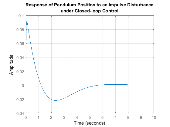
From examination of the figure above, it is apparent that the response of the system is now stable. However, the pendulum position overshoots past the required limit of 0.05 radians and the settle time is on the verge of being greater than the requirement of 5 seconds. Therefore, we will now concentrate on improving the response. We can use the Control System Designer to see how changing the controller gain and the location of the zeros affects the system's frequency response plots. In this case, increasing the controller gain increases the system's phase margin which should help reduce the overshoot of the response. Furthermore, trial and error shows that moving one of the zeros farther to the left in the complex plane (more negative) makes the response faster. This change also increases the overshoot, but this is offset by the increase in gain. Experimentation demonstrates that the following controller satisfies the given requirements.
(7)
Modify your m-file as shown and re-run at the command line to generate the impulse response plot given below.
K = 35;
C = K*(s+1)*(s+2)/s;
T = feedback(P_pend,C);
t = 0:0.01:10;
impulse(T, t), grid
title({'Response of Pendulum Position to an Impulse Disturbance';'under Closed-loop Control'});
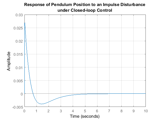
Our response has met our design goals. Feel free to vary the parameters further to observe what happens. Note that it is also possible to generate the system's response to an impulse disturbance from within the Control System Designer. Including the integrator with the controller, rather than with the plant, as is proper will result in the numerical abberation observed above, but will not significantly affect the impulse response generated by MATLAB.
What happens to the cart's position?
At the beginning of this page, a block diagram for the inverted pendulum system was given. The diagram was not entirely complete.
The block representing the response of the cart's position  was not included because that variable is not being controlled. It is interesting though, to see what is happening to the
cart's position when the controller for the pendulum's angle is in place. To see this we need to consider the full system block diagram as shown in the following figure.
was not included because that variable is not being controlled. It is interesting though, to see what is happening to the
cart's position when the controller for the pendulum's angle is in place. To see this we need to consider the full system block diagram as shown in the following figure.

Rearranging, we get the following block diagram.

In the above, the block is the controller designed for maintaining the pendulum vertical. The closed-loop transfer function  from an input force applied to the cart to an output of cart position is, therefore, given by the following.
(8)
Referring to the Inverted Pendulum: System Modeling page, the transfer function for  is defined as follows.
(9)![$$P_{cart}(s) = \frac{X(s)}{U(s)} = \frac{ \frac{ (I+ml^2)s^2 - gml } {q}
}{s^4+\frac{b(I+ml^2)}{q}s^3-\frac{(M+m)mgl}{q}s^2-\frac{bmgl}{q}s}
\qquad [ \frac{m}{N}] $$](Content/InvertedPendulum/Control/Frequency/html/InvertedPendulum_ControlFrequency_eq15167269722217001217.png)
where,
(10)![$$q=[(M+m)(I+ml^2)-(ml)^2]$$](Content/InvertedPendulum/Control/Frequency/html/InvertedPendulum_ControlFrequency_eq13265040714817152519.png)
Adding the following commands to your m-file (presuming and are still defined) will generate the response of the cart's position to the same impulsive disturbance we have been considering.
P_cart = (((I+m*l^2)/q)*s^2 - (m*g*l/q))/(s^4 + (b*(I + m*l^2))*s^3/q - ((M + m)*m*g*l)*s^2/q - b*m*g*l*s/q);
T2 = feedback(1,P_pend*C)*P_cart;
T2 = minreal(T2);
t = 0:0.01:10;
impulse(T2, t), grid
title({'Response of Cart Position to an Impulse Disturbance';'under Closed-loop Control'});
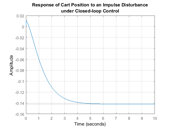
The command minreal effectively cancels out all common poles and zeros in the closed-loop transfer function. This gives the impulse function better numerical properties. As you can see, the cart moves in the negative direction and stabilizes at about -0.14 meters. This design might work pretty well for the actual controller, assuming that the cart had that much room to move. Keep in mind that this was pure luck. We did not design our controller to stabilize the cart's position, the fact that we have is a fortunate side effect.
