


Inverted Pendulum: Simscape Modeling
Contents
Physical Setup
In this section we show how to build the inverted pendulum model using the physical modeling blocks of Simscape Multibody. The blocks in the Simscape library represent actual physical components; therefore, complex multibody dynamic models can be built without the need to build mathematical equations from physical principles as was done by applying Newton's laws to generate the model implemented in Inverted Pendulum: Simulink Modeling.
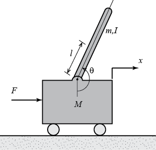
The system parameters are defined as follows:
(M) mass of the cart 0.5 kg
(m) mass of the pendulum 0.2 kg
(b) coefficient of friction for cart 0.1 N/m/sec
(l) length to pendulum center of mass 0.3 m
(I) mass moment of inertia of the pendulum 0.006 kg.m^2
Create world frame and basic configuration
Open a new Simscape Multibody model by typing smnew in the MATLAB command window. A new model opens, as shown below, with a few commonly used blocks already in the model. The PS-Simulink and Simulink-PS blocks define the boundary between Simulink input/output models where the blocks are evaluated sequentially and Simscape models where the equations are evaluated simultaneously.

To configure basic settings in the model, carry out the following:
- Double-click on the Mechanism Configuration block and set Gravity to "[0 0 -9.81]", this represents an acceleration due to gravity of
 acting along the global -Z direction
- Open the Solver Configuration block and ensure that the Use local solver checkbox is not selected.
- Type CTRL-E to open the Configration Parameters dialog
- On the Solver pane, ensure that Type is set to "Variable-Step" and that Solver is set to "auto", also set the Stop time to "10"
Assemble base plane and cart
We will model the cart as a point mass moving along an axis. We use the World Frame to define the axis along which the cart will travel.
- Connect the B port of the Rigid Transform block to the W port of the World Frame
- Double-click on the Rigid Transform block
- In group Rotation, set Method to "Standard Axis", Axis to "+Y" and Angle to "90 deg"
- Rename the Rigid Transform block to "Transform Vehicle Axis"
![]()
Tips for adding blocks:
- Use Quick Insert to add the blocks. Click in the diagram and type the name of the block (use the letters in bold below). A list of blocks will appear and you can select the block you want from the list.
- After the block is entered, a prompt will appear for you to enter the parameter. Enter the variable names as shown below.
- To rotate a block or flip blocks, right-click on the block and select an option from the Rotate & Flip menu.
- To show the parameter below the block name, see Set Block Annotation Properties in the Simulink documentation.
Add the following blocks:
* Prismatic Reference
* Scope
* Pulse Generator
For the Pulse Generator, double-click on the block and set Period to "10", Amplitude to "1000", Pulse Width to "0.01", and Phase delay to "1".
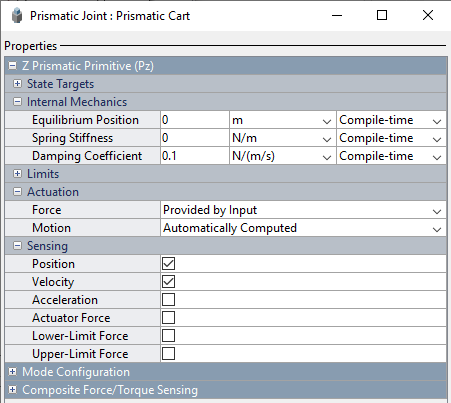
The Prismatic Joint allows only one translational degree of freedom. The Prismatic Joint will be actuated by a force input.
- Double-Click on the Prismatic Joint to open the dialog box
- In group Internal Mechanics, set Damping Coefficient to "0.1 N/(m/s)"
- Under group Actuation, set the Force to "Provided by Input"
- In group Sensing, select Position and Velocity
- Rename the Prismatic Joint to "Prismatic Cart"
The Prismatic Joint next needs to be connected to the rest of the model.
- Connect the B port of Prismatic Cart to the F port of block Transform Vehicle Axis
- Connect the F port of Prismatic Cart to the R port of the solid block
- Rename the Pulse Generator block to "Disturbance" and connect the output of the "Disturbance" to the Simulink-PS Converter block that is already in the diagram
- Connect the output of the Simulink-PS Converter block to the force input of Prismatic Cart
- Double-click on this signal and name it "Force"
- Double-click on the Simulink-PS Converter block and set Input signal unit to "N" for newtons
- Make a copy of the PS-Simulink block
- Double-click on one PS-Simulink block and set Output signal unit to "m", and connect that block to the p port of the Prismatic Cart block
- Double-click on the other PS-Simulink block, set the Output signal unit to "m/s" and connect it to the v port of the Prismatic Cart block
- Connect both PS-Simulink blocks to the Scope
- Name the signal from the p port "x Cart"
- Name the signal from the v port "v Cart"
Since we are modeling the sliding cart as a point mass, only the mass will affect the simulation results.
- Double-click on the solid block
- Set parameter Dimensions to "[0.2,0.04,0.6]" so that the longest dimension points along the direction of travel.
- In group Inertia, set Type to "Point Mass" and Mass to "0.5 kg"
- In group Graphic, under Visual Properties set Color to "[0.8 0.45 0]"
- Rename the block to "Cart"

The model at this point should now appear as follows.
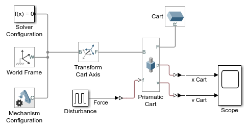
Running a simulation (type CTRL-T or press the green arrow run button), the resulting plot shows both the distance traveled by the cart as well as its velocity.

Pendulum subsystem and connecting the cart to the pendulum
Add the following blocks to the model:
- A Rigid Transform block
- A Brick Solid block (Solid block prior to R2019b)
- A Revolute Joint
To define the axis of rotation for the pendulum:
- Connect the B port of the new Rigid Transform block to the F port of Prismatic Cart
- Connect the F port of the new Rigid Transform block to the B port of the new Revolute Joint block
- Double-click on the new Rigid Transform block
- In group Rotation, set Method to "Standard Axis", Axis to "+X", and Angle to "90 deg"
- Rename the block "Transform Pendulum Pivot" the revolute
![]()
To define the degree of freedom of rotation for the pendulum:
- Rename Revolute Joint to "Revolute Pendulum"
- Connect F port of Revolute Pendulum to R port of Brick Solid block (Solid block prior to R2019b)
To model the pendulum:
- Double-click on the Brick Solid block
- In group Geometry, set Dimensions to "[0.6 0.03 0.05] m"
- In group Inertia, set Type to "Point Mass" and Mass to "0.2 kg"
- In group Graphic, under Visual Properties set Color to "[0.25 0.4 0.7]"
- Press OK, and rename the block to "Pendulum"

To model the connection point to the cart:
- Double-click on the Pendulum block
- In group Frames, click on the + next to New Frame, this opens the frame definition interface
- Click on the small face of the brick facing you (along positive x direction) to select it
- In section Frame Origin, select radio button Based on Geometric Feature
- Click the Save button at the bottom of the dialog box
- Change the name of "Frame1" to "B"
- Unselect the checkbox for Show Port R
- Click OK
- Connect the B port of Pendulum to the F port of "Transform Pendulum Pivot"

The resulting model should appear as follows:

Running a simulation (type CTRL-T or press the green arrow run button), the following plot is generated, where one can see that the addition of the pendulum alters the cart behavior both in its distance traveled as well as its velocity.

Selecting outputs for controller and angle conversion
We now need to measure the angle and angular velocity of the pendulum:
- Double-click on "Revolute Pendulum"
- In group Z Revolute Primitive (Rz) under Sensing, select checkboxes for Position and Velocity
- Make two copies of the PS-Simulink converter block
- Double-click on one PS-Simulink block and set Output signal units to "rad"
- Connect that PS-Simulink block to the q port on Revolute Pendulum
- Double-click on the other PS-Simulink block and set Output signal units to "rad/s"
- Connect that PS-Simulink block to the w port on Revolute Pendulum
We need to limit the measured angle to stay between -pi and pi radians.
- Add a Subsystem block to your model
- Rename the Subsytem block "Wrap Angle"
- Double-click to enter the Wrap Angle subsystem
In this subsystem we will add pi radians to the measurement, find the remainder when the signal is divided by 2*pi, and then subtract pi radians.
- Rename the input block "q"
- Delete the signal connection between the inport and the outport
- Add a Bias block to the model
- Set parameter Bias to "pi"
- Connect the q block to the Bias block
- Add a Math Function block to the model
- Double-click on the Math Function block and set Function to "rem"
- Connect the output of Bias to the first input of the Math Function block
- Add a Constant block to the model
- Set parameter Constant to "2*pi"
- Connect the Constant block to the second input of the Math Function
- Make a copy of the Bias block
- Set parameter Bias in the new block to "-pi"
- Connect Math Function output to the input of the new Bias block
- Connect the output of the new Bias block to the outport
- Rename the outport "qwrap"
- Go up one level in the diagram and rename the subsytem "Wrap Angle"
Here you can see the resulting subsystem for wrapping the angle

We will plot the new signals on a Scope
- Connect PS-Simulink output for the q measurement of Revolute Pendulum to the input of Wrap Angle
- Add a new Scope
- Connect the qwrap output of Wrap Angle to the new Scope and change the name of this signal to "q pendulum"
- Connect the PS-Simulink output for the w measurement of Revolute Pendulum to the new Scope and change the name of this signal to "w pendulum"
The resulting model should appear as follows:
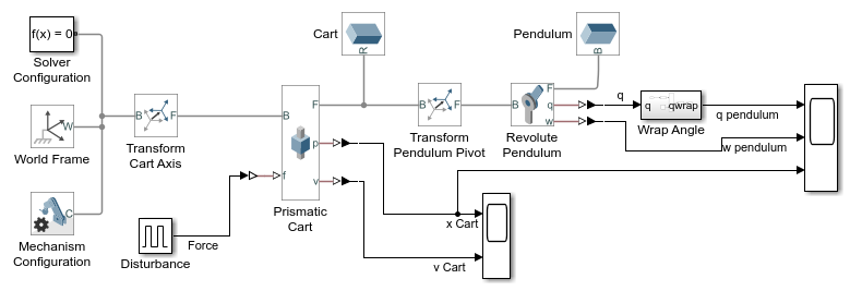
Running a simulation (type CTRL-T or press the green arrow run button), the followings plot are generated. The motion of the cart is the same as before, but now we can see the motion of the pendulum. The associated animation shown below is also generated.


Create subsystem for pendulum and cart
We have now successfully created all the elements of the inverted pendulum system. We will convert this into a subsystem.
- Click once in the diagram (but not on a block) and press CTRL-A to select all blocks
- Hold the Shift key and click on the Disturbance block and each Scope to unselect those blocks
- Press CTRL-G to create a subsystem
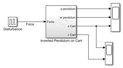
- Rename the subsystem "Inverted Pendulum on Cart"
Your model should now appear as shown:
Closed-loop setup
We will now add blocks for open and closed-loop testing.
Add the following blocks:
- Subtract
- PID Controller
- Constant
- Manual Switch
- Sum
The Disturbance also will be added to the control signal.
- Delete the signal connecting Disturbance to the cart subsystem
- Connect the output of the sum block to the Force input of the cart subsystem
- Connect Disturbance to the bottom + port of the Sum block
We wish to manually select open or closed-loop behavior.
- Connect the Manual Switch output to the + input of the Sum block
- Connect the Constant block to the lower input of the Manual Switch, then set the parameter Constant to "0" and rename block "No Force"
- Connect the output of the PID Controller to the upper input of Manual Switch
- Connect the Subtract block output to the input of PID Controller
We will close the loop to control the pendulum angle.
- Connect q pendulum output of the cart subsystem to the - port of the Subtract block
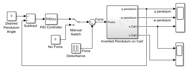
- Make a copy of the Constant block and connect it to the + port of the Subtract block and rename the block "Desired Pendulum Angle"
Your model should now appear as follows. The output of the simulation is unchanged from prior results when in open-loop mode.

Controller implementation
We will now implement the PID control gains developed in the Inverted Pendulum: PID Controller Design page.
- Double-click on the PID Controller block
- Set parameter Proportional (P) to "100"
- Set parameter Integral (I) to "1"
- Set parameter Derivative (D) to "20"
Double-click on Manual Switch until the input from the PID Controller is selected.
Running a simulation produces the following two plots show the controlled response of the system. After the initial impact the controller was able to quickly bring down the pendulum angle to zero and the pendulum velocity is also zero. The cart moves slowly and with a constant velocity in the negative X direction to keep the pendulum balanced.


You can download the final Simscape model created here by right-clicking here and then selecting Save link as ....
