Activity 6 Part (b): PI Control of a DC Motor

Key Topics: Pulse-Width Modulation, PI Control, Pole Placement, Steady-State Error, Disturbance Rejection, Saturation, Integrator Wind-up, Embedded Control

Equipment needed
Purpose
Control requirements
System identification experiment
Controller design via algebraic pole placement
PI controller implementation
Robustness to disturbances
Embedded Control

Equipment needed

Arduino board (e.g. Uno, Mega 2560, etc.)
Breadboard
DC motor with quadrature encoder
Battery (lantern battery for example)
Diode
Transistor (MOSFET)
Jumper wires

In this activity we will design and implement a speed controller for a simple DC motor. In particular, we will choose and tune the gains of a PI controller based on the effect of the gains on the system's closed-loop poles while accounting for the inherent uncertainty in our model. We will design the controller to achieve a desired level of transient response and will examine in detail the steady-state error produced by the resulting closed-loop system, including in the presence of a constant disturbance. More details regarding other approaches to motor speed control and alternative control design techniques can be found from the home page of these tutorials.

The motor's angular speed is estimated employing a quadrature encoder. The encoder pulses are counted on the Arduino board via two of the board's Digital Inputs. One of the board's Digital Outputs is also employed to switch a transistor on and off, thereby connecting and disconnecting the motor to a DC voltage source. The Arduino board communicates the recorded data to Simulink for visualization and analysis. The logic for estimating the motor's speed based on encoder counts and the logic for controlling the motor's speed is implemented within Simulink. Initially this logic is run on the host computer, but later we download all of the logic to the Arduino board.

Purpose

The purpose of this activity is to build intuition regarding the design and implementation of a PI controller for the speed control of a DC motor in the presence of an array of real-world complications. Specifically, we will consider how to design the controller when we have an uncertain plant model and are limited in the amount of control effort we can supply. Furthermore, we will analyze our system's performance in the presence of unwanted exogenous inputs, which in this case will be a constant disturbance.

Control requirements

The plant $P$ for this activity will be the same armature-controlled DC motor we explored in Activity 6a.

At a fundamental level, the voltage source (V) applied to the motor's armature is its input and the rotational speed of the shaft $d\theta/dt$ is the output. Since in practice we are employing a Pulse-Width Modulation (PWM) approach to control, we will treat our control input as the PWM signal's duty cycle (percent of the PWM period for which the motor is "on"). The control input to the motor will be determined via a PI control law $C(s)$ acting on the error between the commanded and measured motor speed. In the previous activity, we generated a first-order model of the plant $P(s)$ based on the motor's step response. In that activity, we investigated the processing needed for estimating the motor's speed, including a low-pass filter to "smooth" the quite noisy speed estimate. In this context, our closed-loop system would have the following form where the motor's speed is the true output, but significant processing (via $H(s)$ ) is needed to generate the measured speed employed for feedback.

Since we have no means for measuring the motor's true speed, we will rather consider our closed-loop system to have the following format where our plant $P'(s)$ includes the dynamics of the signal processing. We will determine a model for $P'(s)$ in the same blackbox manner we did in Activity 6a (except here we will include the filtering in our "plant").

The specific transient controller requirements that we will design for are given below. If you are employing a physical motor significantly different than what we will employ here, you may wish to alter the given requirements accordingly. We will also analyze the steady-state behavior of the system, including in the presence of a constant disturbance.

2% settling time less than 1 second
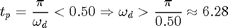
Peak time less than 0.50 seconds
Maximum overshoot less than 20%

System identification experiment

In this activity we will employ the same hardware setup we used in the first part of the activity. Before moving on to the control portion of the activity, we will first generate a blackbox model for the motor as we did in Activity 6a.

Hardware setup

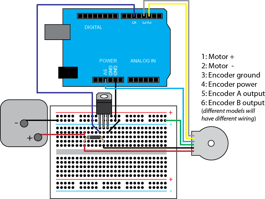
In this experiment we will control our motor through one the board's digital outputs. Specifically, the digital output will be used to switch a transistor on and off, thereby connecting and disconnecting the motor to the battery power source. In order to prevent the motor's back emf from causing damage, we will include a diode in parallel with our motor.

In the schematic shown, we employ a power MOSFET where the board drives the Gate pin. When voltage is supplied to the Gate, it closes the circuit between the Source and Drain pins. One possible choice of power MOSFET is the IRF1520 whose datasheet can be found here. For our diode, we will employ the general purpose 1N4007 whose datasheet can be found here.

We are able to achieve approximately continuous control of the motor's speed using only a DC source by employing Pulse-Width Modulation (PWM). Recall, a PWM approach alternately turns the motor "on" and "off". Since the motor has dynamics (inertia, friction, etc.), it doesn't instantaneously reach top speed when turned on and doesn't immediately come to a stop when turned off; it takes time for the motor to react. This can be used to our advantage if the PWM frequency is sufficiently fast. It's as if the motor is filtering the PWM command. In this way, the speed of the motor can be controlled continuously by varying the percent of time the PWM signal is "on" compared to the overall period (the duty cycle). Further details on PWM can be found in Activity 1b and Activity 4.

We will also employ the Arduino board for sensing the angular speed of the motor. Specifically, we will employ a quadrature encoder. One motor with Hall-effect encoder that could be used for this activity can be found here, though there are many other choices. This particular motor can be driven by a 6-V lantern type battery. The encoder provides 48 counts per revolution (if you count both rising and falling edges). The motor also includes a gearbox so that the Hall-effect sensor generates 1633 counts per revolution of the output shaft of the gearbox. Ultimately, the gearbox is not necessary for this activity and a version of this motor can be purchased without the gearbox for less money here. Various accessories for the motor (brackets, wheels, etc.) can be found from the same website.

The setup of the motor with encoder and its connection to the Arduino board is shown below. The color band on the diode indicates its cathode. The Gate, Source, and Drain pins of the MOSFET can be deduced from its orientation in the given figure.

Software setup

In this experiment, we will employ Simulink to control the motor through the switching of the transistor, to read the encoder output, and to plot the data in real time. In particular, we will employ the IO package from the MathWorks. For details on how to use the IO package, refer to the following link.

To generate our plant model, we will employ the same Simulink model we employed in the first part of this activity. This model is shown below and can be downloaded here. Further details on its construction can be found in Activity 6a.

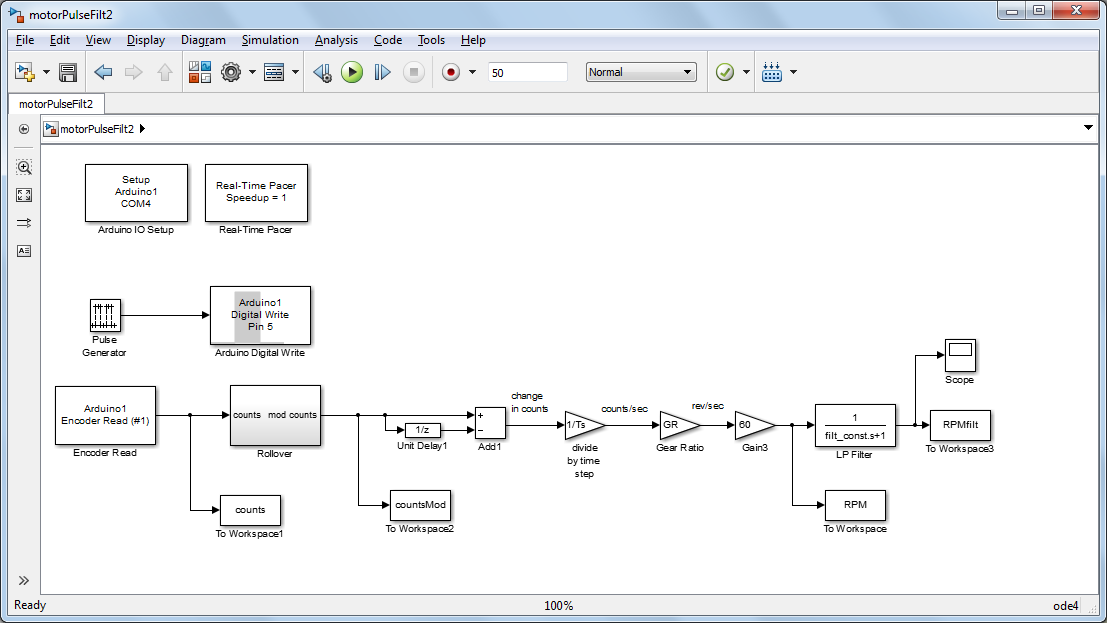
Before we run this model, we need to define several parameters used in the model. You can define the following parameters at the MATLAB command line, or can run a script .m file that includes their definition. Your gear ratio may be different than what is employed here depending on your specific model of motor. You may also need to change the COM port specified in the Arduino IO Setup block.

Ts = 0.02;              % model sample time in seconds
filter_const = 5*Ts;    % time constant of the first-order filter
GR = 1/1633;            % gear ratio

After running the above model and plotting the filtered output, you should observe a speed response plot like the one shown below.

From inspection, we can see that the response has the appearance of a first-order step response. Therefore, we will fit a first-order model to the data in the same manner that we did in Part (a) of this activity. The only difference here is that we will include the filter dynamics as part of our "plant" and we will consider our input to be duty cycle (a percentage) rather than input voltage.

(1) $P'(s) = \frac {\dot{\Theta}(s)}{DC(s)} = \frac{K}{\tau s + 1} \qquad [RPM]$

From inspection, the steady-state speed reached by the motor is approximately 170 RPM. Since this is for a 5-Volt step, we can consider our input to be a duty cycle equal to 1 (100%), and the DC gain for the model is simply $K = 170$ RPM. Recall that a time constant defines the time it takes a process to achieve 63.2% of its total change. Therefore, we can estimate the time constant based on the time it takes the motor speed to reach $0.632 \times 170 \approx 107$ RPM. Since this appears to occur at 1.23 seconds and the input appears to step at 1.07 seconds, we can estimate the motor's time constant to be approximately 0.16 seconds. Therefore, our blackbox model for the motor is the following.

(2) $P'(s) = \frac {\dot{\Theta}(s)}{DC(s)} = \frac{170}{0.16s + 1} \qquad [RPM]$

Controller design via algebraic pole placement

In this section, we will initially design our PI controller algebraically. That is, we will choose the control gains $K_i$ and $K_p$ to place the closed-loop poles in some desired locations, $C(s) = K_p + K_i/s$ . Therefore, we must first determine the closed-loop transfer function for the system as defined above.

(3) $T(s) = \frac{Y(s)}{R(s)} = \frac{C(s)P'(s)}{1+C(s)P'(s)} = \frac{\frac{(K_ps + K_i)170}{s(0.16s+1)}}{1 + \frac{(K_ps + K_i)170}{s(0.16s+1)}} = \frac{170(K_ps+K_i)}{0.16s^2+(1+170K_p)s+170K_i}$

By inspection, we see that the closed-loop system is second-order with a zero. The system does not match the canonical form shown below because of the presence of the zero.

(4) $G_{canon}(s) = \frac{\omega_n^2}{s^2+2\zeta\omega_ns+\omega_n^2}$

Despite the presence of the zero, we will initially treat our system as if it did have a canonical form. Therefore, our initial design will not reflect the true behavior of our closed-loop system with zero (not to mention the uncertainty in the plant model). Despite these limitations, this design will provide a good starting point and will prove qualitatively helpful to us in the tuning of our controller.

Matching the denominator of our closed-loop transfer function $T(s)$ to the canonical form above, we get the following relationships between control gains and desired closed-loop pole locations (as indicated by $\sigma$ , $\omega_d$ , etc.).

(5) $\frac{1 + 170 K_p}{0.16} = 2\zeta\omega_n = 2\sigma$

(6) $\frac{170 K_i}{0.16} = \omega_n^2$

We can then choose our control gains in an attempt to achieve closed-loop pole locations that satisfy our original system requirements on settling time, peak time, and maximum overshoot. In this process we will use the following expressions, which again assume a canonical second-order underdamped system (which we don't have).

2 $\%$ settling time: $t_s \approx \frac{4}{\sigma}$
Peak time: $t_p=\frac{\pi}{\omega_d}$
Maximum percent overshoot: $M_p = e^{-\zeta\pi/\sqrt{1-\zeta^2}} \times 100\%$

Based on the given requirements and assumed relationships shown above, we can determine the desired poles locations that in turn determine our choice of control gains $K_p$ and $K_i$ . In order to satisfy our settling time requirement, we place the following constraint on $\sigma$ .

(7) $t_s \approx \frac{4}{\sigma} < 1 \Rightarrow \sigma > 4$

Now examining our peak time requirement, we determine a constraint on $\omega_d$ .

(8) $t_p = \frac{\pi}{\omega_d} < 0.50 \Rightarrow \omega_d > \frac{\pi}{0.50} \approx 6.28$

And finally, our maximum percent overshoot requirement places a constraint on $\zeta$ .

(9) $M_p = e^{-\zeta\pi/\sqrt{1-\zeta^2}} < 0.20 \Rightarrow \zeta > \sqrt \frac{(\ln 0.20)^2}{\pi^2 + (\ln 0.20)^2} \approx 0.456$

If we choose our gains to meet the three above constraints, our closed-loop system will not be guaranteed to meet the associated requirements because our system is not canonical (it has a zero) and because our actual physical plant won't match our theoretical model. That being said, the above relationships are still useful in qualitatively guiding the tuning of the control gains, as we will eventually demonstrate.

To help visualize the above requirements, we will map them to the complex s-plane as shown below. Specifically, $\sigma$ corresponds to the real part of our poles, $\omega_d$ corresponds to the imaginary part of our poles, and $\zeta$ maps to the angle $\beta$ via the relation $\zeta = \cos \beta$ . Therefore, we need $\beta < \cos^{-1}(0.4556) \approx 62.3^{\circ}$ . The shaded region corresponds to the pole locations that satisfy all three requirements.

Based on these requirements, we can choose the closed-loop poles to equal $-5 \pm 10j$ . We could also choose the poles to meet the requirements with greater margin, the only drawback is that making the system "faster" (smaller settling time and smaller peak time) tends to come at the cost of increased control effort, something we will discuss when we implement our controller. Now looking back at our original closed-loop transfer function, we can pick our control gains $K_p$ and $K_i$ to achieve the chosen closed-loop pole locations, where $\sigma$ equals 5 and $\omega_d$ equals 10.

(10) $\frac{1 + 170K_p}{0.16} = 2\sigma \Rightarrow K_p = \frac{2(5)(0.16) - 1}{170} \approx 0.0035$

(11) $\frac{170K_i}{0.16} = \omega_n^2 = \sigma^2 + \omega_d^2 \Rightarrow K_i = \frac{(5^2 + 10^2)(0.16)}{170} \approx 0.12$

We can now implement our controller as designed.

PI controller implementation

We will develop and implement our control algorithm within Simulink. We can begin with the model that we used previously for identifying a model for our plant. Starting from this model, we can add a PI compensator as shown below, where the reference speed command will be a step of magnitude 130 RPM (chosen to be less than the motor's maximum speed, 170 RPM in this case). This reference then subtracts the plant's output, which in this case is the filtered estimate of the motor's speed. The output of this summing junction, the measured speed error, is then fed into the control algorithm. The controller in this case has two terms, the P term which is proportional to the error via the gain $K_p$ , and the I term which is proportional to the integral of the error via the gain $K_i$ . The sum of these two terms is the control input to the plant. The control input is specifically the duty cycle of the PWM signal applied to the motor. In order to generate this PWM signal, the Arduino Digital Write block that was being employed previously needs to be replaced by an Arduino Analog Write block (still set to Pin 5). The name of this block is a bit of a misnomer since it generates a PWM signal which is still a digital output. Since the block encodes the duty cycle as an 8-bit number, it accepts inputs from 0 to 255, corresponding to a 0% and a 100% duty cycle, respectively. In addition to the Gain block that converts the duty cycle command to bits, we have also included a saturation block to capture the fact that the duty cycle cannot be less than 0% or greater than 100%. If we employed an H-bridge, we could also drive the motor backwards (allowing a "negative" control input), but in this activity we only command the motor to spin in one direction. You can create the model yourself, or download it here.

Once we have created this model, it can then be run to observe the performance of the controller we just designed. Prior to running the model, make sure to define $K_p$ and $K_i$ (in addition to Ts, filter_const, and GR). Just out of interest, let's first run our model with only a P controller. That is, set $K_p = 0.0035$ and let $K_i = 0$ . Under these conditions, our closed-loop system generates the following response to a step reference of 130 RPM.

Since we didn't perform our controller design for a P controller, we don't know exactly what to expect in terms of the transient response. However, it is interesting to inspect the steady-state response. Here we see that the steady-state speed settles somewhere below 60 RPM which is quite different than the 130 RPM reference that was commanded. The presence of such a level of steady-state error, however, is not surprising since our system is type 0 under P control. Let us now add the integral term we designed earlier, $K_i = 0.12$ . The system response that is produced for this PI controller is shown below.

Examining the resulting steady-state response, the motor's speed seems to settle out near the commanded reference of 130 RPM. This is expected since the addition of the integral term to our controller increased the system's type to 1. The transient response, however, isn't exactly what we designed for. Specifically, we designed our controller to place the system's closed loop poles at $-5 \pm 10j$ . If these poles belonged to a canonical second-order system, we would then expect the system's step response to have the following characteristics:

(12) $t_s \approx \frac{4}{\sigma} = \frac{4}{5} = 0.8\ \mbox{seconds}$

(13) $t_p = \frac{\pi}{\omega_d} = \frac{\pi}{10} \approx 0.314\ \mbox{seconds}$

(14) $\%M_p = e^{\frac{-\zeta\pi}{\sqrt{1-\zeta^2}}} \times 100\% = e^{\frac{-0.53\pi}{\sqrt{1-0.53^2}}} \times 100\% \approx 14\%$

Inspection of the recorded motor speed demonstrates that the system is more oscillatory (larger overshoot and settling time) than designed for. Also, the peak time is larger than designed for. There are several obvious reasons for the noted discrepancy. One is the fact that our system is not canonical, it has a zero. This increased oscillation could be explained by the zero, though zeros tend to decrease peak time, not increase it, as we have observed here. Another likely contributing factor is the limited accuracy of our model. We fit a first-order model to the step response data, but the true system likely has higher-order dynamics and nonlinearities that are not modeled. Furthermore, our model is continuous, when in fact we have a digital implementation. If the sampling time is very fast compared to the dynamics of the system, then neglecting the sampling effects is a reasonable thing to do. In our case, our sampling time (Ts = 0.02 seconds) is significant compared to the speed of our system. Despite all of these effects, the single most likely cause of the observed discrepancy is the fact that our control input is saturating. Below is shown the duty cycle command being sent to the motor system.

Inspection of the above shows that as the motor speed oscillates, the control effort periodically saturates (the duty cycle cannot be greater than 100%). One effect of the saturation is that the speed of response will be less than if there was no saturation, less control effort generally corresponds to slower response. This somewhat explains the larger than expected peak time that was observed. Another effect of the saturation is that it can make the system more oscillatory in the presence of an integral controller. This effect can be understood by considering how the integral term of our controller works.

Integrator windup

The integrator term of the controller integrates the feedback error over time. Thinking of the integrator as summing the area under a graph of the error, we can see that when the error is positive the integral term gets larger and when the error is negative the integral term gets smaller. The figure below shows an underdamped step response like we have here. Initially the motor is at rest and the commanded reference is 130 RPM, therefore, the error is positive and the integral term quickly integrates the first positive green area shown in the figure below. This quick increase in the integral term (along with the proportional term) causes the control effort in this case to saturate almost immediately as indicated by the graph of duty cycle shown above. The thing about the integrator is that it keeps building and in essence "asking" for more control effort even though the control signal has saturated and can't provide any more effort. Once the measured motor speed exceeds the 130 RPM, the error then becomes negative and the first red area in the graph below begins to subtract away from the area that has been accumulated by the integrator term. Since the integrator term built up a significant amount of positive "area," the control effort continues to be positive (and saturated) well after the point at which the motor has exceeded the 130 RPM commanded reference and actually needs to slow down. The control basically has to wait for the first red area to subtract away enough of the green area that has already been accumulated before the integral term of the controller will decrease to a sufficient degree that the motor will actually start to slow down.

This effect is known as Integrator windup and can lead to excessive lag and oscillation in our closed-loop system's performance. There are different techniques for addressing this effect. Some Anti-windup measures include turning the integrator "off" such that it stops accumulating at the point the control effort saturates. Another technique is to reset the value of the integrator to zero at which point the error switches sign. For now, we will try to tune our control gains to avoid the saturation. Later we will observe the effect of this integrator windup in a more dramatic fashion.

If we wished to decrease the effect of the integrator windup, the simplest solution would be to decrease the integral control gain $K_i$ . Recalling the relations between our closed-loop denominator and the form of a canonical second-order system, repeated below, we can see that decreasing $K_i$ in turn decreases $\omega_n$ . If we left $K_p$ unchanged, then $\sigma$ would be unchanged and $\omega_d$ would decrease as well.

(15) $\frac{1 + 170K_p}{0.16} = 2\sigma$

(16) $\frac{170K_i}{0.16} = \omega_n^2 = \sigma^2 + \omega_d^2$

A decrease in $\omega_d$ should correspond to an increase in $t_p$ based on the canonical relation, $t_p = \pi/\omega_d$ . Even though we do not have a canonical second-order system, and even though our model is quite uncertain, these relationships are often helpful in guiding the qualitative effect of changes in control gains. The effect of increasing $t_p$ , making the system respond more slowly, should also help avoid the saturation problem. Furthermore, since the previously observed $t_p$ was less than the requirement of 0.5 seconds, we should be able to decrease $K_i$ some and still meet our $t_p$ requirement. A decrease in $\omega_d$ while keeping $\sigma$ unchanged also corresponds to a decrease in $\beta$ (an increase in $\zeta$ ), which should help reduce the overshoot. This change to the system's previous response is also needed to meet the given requirements.

After some trial and error, we settle on reducing the integral gain to $K_i = 0.04$ while leaving the proportional gain as $K_p = 0.0035$ . The resulting closed-loop performance can be seen below. The noise on the speed estimate makes it a little difficult to determine whether or not the given requirements are met, but we will attempt to visualize a smooth line fitted through the noisy data. By inspection, it appears that the peak time is less than 0.5 seconds, the settling time is less than 1 second, and the maximum percent overshoot is less than 20%. The control effort does appear to saturate for a brief time. Decreasing $K_i$ slightly further would avoid the saturation, though the saturation isn't necessarily a problem in this instance, other than indicating that the power source (the battery) may be depleted more quickly.

Robustness to disturbances

So far we have designed a PI controller in the presence of a variety of real-world complications including uncertainties in the plant model and limits on the available control effort. Another factor that often must be considered in the implementation of control systems is the effect of unwanted inputs, such as disturbances and noise. In this section we will consider that our motor is subject to an unwanted load torque disturbance $T_L$ as shown below. In order to model the entry of this torque into the model, we split our motor model into its electrical dynamics and its mechanical dynamics. As the electrical dynamics are generally much faster than the mechanical dynamics, we will model the electrical dynamics as a simple gain, i.e. as static. We will also neglect the effect of the motor's back emf.

When we have a linear model and controller, as we have here, we can analyze a system subject to multiple simultaneous inputs using the property of Superposition. This property allows us to analyze the system's response to the individual inputs separately and then to consider their total effect as simply the sum of their individual effects. We will illustrate this approach in the following. We previously found the closed-loop transfer function from the reference to the output. This transfer function is repeated below in terms of the parameters shown in the above block diagram.

(17) $G_R(s) = \frac{Y(s)}{R(s)} = \frac{\dot{\Theta}_m(s)}{\dot{\Theta}_{ref}(s)} = \frac{K_eK_m(K_ps+K_i)}{\tau s^2+(1+K_eK_mK_p)s + K_eK_mK_i}$

In a similar manner, we can find the transfer function from the disturbance to the output as shown below.

(18) $G_D(s) = \frac{Y(s)}{D(s)} = \frac{\dot{\Theta}_{m}(s)}{T_L(s)} = \frac{P_m(s)}{1+C(s)P_e(s)P_m(s)} = \frac{\frac{K_m}{\tau s+1}}{1 + \frac{K_eK_m(K_ps + K_i)}{s(\tau s+1)}} = \frac{K_m s}{\tau s^2+(1+K_eK_mK_p)s+K_eK_mK_i}$

Applying the property of superposition, the total output of the motor under simultaneous application of a reference input and a disturbance input is then as follows.

(19) $\dot{\Theta}_{m}(s) = \frac{K_eK_m(K_ps+K_i)}{\tau s^2+(1+K_eK_mK_p)s + K_eK_mK_i}\dot{\Theta}_{ref}(s) + \frac{K_m s}{\tau s^2+(1+K_eK_mK_p)s+K_eK_mK_i}T_L(s)$

For the purposes of this activity, we will simply examine the steady-state error that the closed-loop system will experience under the influence of an approximately constant disturbance load torque. To predict the kind of behavior we expect, we can apply the final value theorem.

(20) $\dot{\theta}_{m,ss} = \lim_{t \rightarrow \infty} \dot{\theta}_m(t) = \lim_{s \rightarrow 0} s\dot{\Theta}_m(s) = \lim_{s \rightarrow 0} s G_D(s)T_L(s)$

For a constant disturbance, $T_L(s) = D/s$ . Therefore, we have the following.

(21) $\dot{\theta}_{m,ss} = \lim_{s \rightarrow 0} s \frac{K_m s}{\tau s^2+(1+K_eK_mK_p)s+K_eK_mK_i} \cdot \frac{D}{s} = \lim_{s \rightarrow 0} \frac{DK_m s}{\tau s^2+(1+K_eK_mK_p)s+K_eK_mK_i} = 0$

Since the steady-state speed output under PI control is zero for a constant disturbance input, we would expect that the steady-state error would also be zero. The output will not deviate from its steady-state value due to the constant disturbance, only the output response due to the reference input will remain in steady-state. Let's test this hypothesis by running our Simulink model with the PI controller we previously designed. After the reference input has stepped, we will add a constant load torque by lightly applying constant pressure to the output motor shaft with our fingers. The resulting motor speed and control effort should appear something like the following.

In the above experiment, the load disturbance is applied between approximately 4 seconds and 7 seconds. By inspection, the motor speed does not deviate from the commanded 130 RPM reference even when this constant disturbance is applied. This agrees with our prediction based on the final value theorem. Looking at the control effort during this experiment, however, we can see that the duty cycle increases slightly between 4 seconds and 7 seconds. This increase in effort generates the additional motor torque needed to counteract the increased load during this time frame.

Now let's increase the run time of our Simulink model to 20 seconds and repeat the above experiment. This time, however, we will apply a sufficient amount of pressure with our fingers to momentarily bring the motor to a full stop. The resulting output for this experiment should appear something like the following.

Inspection of the above shows that the load is applied at applied around 4 seconds and released around 6 seconds. Sufficient torque is applied to bring the motor to a full stop. Once the additional load is removed, the motor speed overshoots the 130 RPM reference and stays at its maximum speed of 170 RPM for about 7 seconds before returning to the level of the commanded reference. This behavior rather dramatically demonstrates the effect of integrator windup we discussed earlier. During the time when the motor is held still, the error is quite large and the integrator "winds up." This build-up in the integrator causes the control effort to become quite large and causes the motor speed to overshoot the commanded reference speed once the motor is released. It then takes quite a while for the negative error to reduce the integrator accumulation and allow the motor to slow down again.

Embedded Control

So far in this experiment, the logic for controlling the motor's speed has been running in Simulink on a host computer. This was accomplished employing the IO package from the MathWorks which in essence includes a specialized blockset and a program running on board the Arduino for communicating between the board and the host computer running Simulink. The advantage of employing the IO package is that it allows us to communicate with the board in real time with ease. Therefore, we can observe and graph the measured output speed (and control effort) during the experiment.

An alternative to running the control logic on the host computer is to instead run the control logic on board the Arduino. This is referred to as "embedding" the control on the microprocessor of the Arduino board. This approach has two advantages. One, since the control software does not have to run under an operating system (i.e. Windows, etc.) that has to address many other (higher priority) tasks, the control program can run faster and achieve faster sampling rates. The other advantage is that Arduino board does not need to be physically connected to the host computer. So, for example, you can create an autonomous ground vehicle that is driven by DC motors such as we have been experimenting with here. Note that if you want to unplug the Arduino board from the host computer, you will then need to provide an alternative power source (a 9-Volt battery, etc.) for the board. In this activity we so far have been powering the board from the host computer through the USB cable.

In order to embed our control logic on board the Arduino, we will use the Arduino Support Package from the MathWorks. More details can be found here. The blockset of this support package is almost identical to those used previously from the IO package. The Arduino Analog Write block is replaced by a PWM block, but the functionality is the same. The block for reading the encoder is also functionally the same as in the IO Package. This block, however, is not part of the standard Arduino Support Package. You can download the model shown with Encoder block included here, or you can learn how to create your own device drivers (including one for reading encoders) here. The reference for this motor is included within the shown model. Alternatively, you could read the reference via an Analog Input. For example, you could specify the motor speed reference by changing the voltage input using a voltage divider with a potentiometer.

Before you run this Simulink model, you need to double-click on the Encoder block and select the Build button in the upper righthand corner to generate the S-function for reading the encoder. This is shown below. The Encoder block shown is set up for a sample time of Ts = 0.02 and reads the quadrature signals on digital pins 2 and 3. If you wished to change these settings you can do so from within the Encoder block. Specifically, you can change the sample time under the Initialization tab, while the pins that the quadrature signal is read from are defined by the parameters pinA and pinB.

The Arduino IO Setup block and the Real-Time Pacer block are no longer necessary, though the model needs to be set to automatically detect the COM port, or must be manually set to the correct COM port. This can be done through the drop-down menu of the model toolbar Tools > Run on Target Hardware > Options.... This is also where the type of board you are using is set. The Scope and To Workspace blocks are no longer employed. This control software can be deployed to the Arduino board by clicking on the icon resembling a serial port connection, or by typing Ctrl+B. This automatically builds and compiles the Simulink model into code that runs in real time on board the Arduino. This process of Autocode Generation is becoming very common in industrial practice.