Activity 6 Part (a): Time-Response Analysis of a DC Motor

Key Topics: Modeling Electromechanical Systems, Time-Response Analysis, System Identification, Filtering, Reduced-order Models, Stiction, Pulse-Width Modulation

Contents

Equipment needed

In this activity we will model a simple DC motor for an input of armature voltage and an output of rotational speed. The motor's angular position (and in turn its speed) is determined by a quadrature encoder. The encoder pulses are counted on the Arduino board via two of the board's Digital Inputs (each digital channel can be either an input or an output). The Arduino board is also used for controlling the speed of the motor. Specifically, one of the board's Digital Outputs is employed to switch a transistor on and off, thereby connecting and disconnecting the motor to a DC Voltage source. The Arduino board will also communicate the recorded data to Simulink for visualization and analysis. The logic for estimating the motor's speed based on encoder counts is implemented within Simulink. In Part (b), the logic for controlling the motor's speed will also be implemented in Simulink.

Purpose

The purpose of this activity is to build intuition regarding the operation of an armature-controlled DC motor. The activity also generates a blackbox model for the motor based on its step response. This type of model is compared to a physics-based model, the details of which can be found here.

Modeling from first principles

In order to generate a physics-based model of the motor, we need to consider a simplified version of its workings. The following figure represents an electric equivalent circuit of the armature and the free-body diagram of the rotor.

For this example, we will treat the voltage source (V) applied to the motor's armature as the input, and the rotational speed of the shaft as the output. For modeling purposes, the rotor and shaft are assumed to be rigid. We further assume a viscous friction model, that is, that the friction torque is proportional to shaft angular velocity.

The following variables represent the physical parameters of the motor.

(J)     moment of inertia of the rotor

(b)     motor viscous friction constant

(Ke)    electromotive force constant

(Kt)    motor torque constant

(R)     armature resistance

(L)     armature inductance

Based on the above assumptions, we arrive at the following transfer function model of a DC motor where the variable K represents both the motor torque constant and the back emf constant (since the two constants are equal when consistent units are employed). For the details of the derivation of this model, please refer to the DC Motor Speed: System Modeling page.

(1)

Time response experiment

In this experiment we will generate a model for an armature-controlled DC motor based on its step response. Therefore, we will generate a model for the motor based on its observed response, without considering the underlying physics of the motor. This is sometimes referred to as a blackbox model or a data-driven model. After we have generated such a model, we will attempt to explain what we have observed based on our understanding of the underlying physics. In this process we will learn how to interface with a DC motor equipped with a quadrature encoder.

Hardware setup

In this experiment we will control our motor through one the board's digital outputs. Since the board cannot supply enough current (only about 40 milliamps) to drive most motors directly, we will use the low-power signal from the board to connect and disconnect the motor to a higher-power source, i.e. a battery. Specifically, the digital output will be used to switch a transistor on and off. When the transistor is turned "on" it will behave like a closed switch thereby completing the circuit and causing the motor to spin. When the transistor is turned "off" it will act like an open switch such that current won't flow through the circuit and the motor will coast to rest. Since the motor is an inductive load, when we attempt to switch the motor off and it continues to spin (due to its inertia) the motor will generate a back emf (a voltage). This back emf can damage our transistor. In order to prevent this back emf from causing damage, we will put a "flyback" diode in parallel with our motor. The diode will only allow current to flow in one direction, thereby protecting the rest of the circuit.

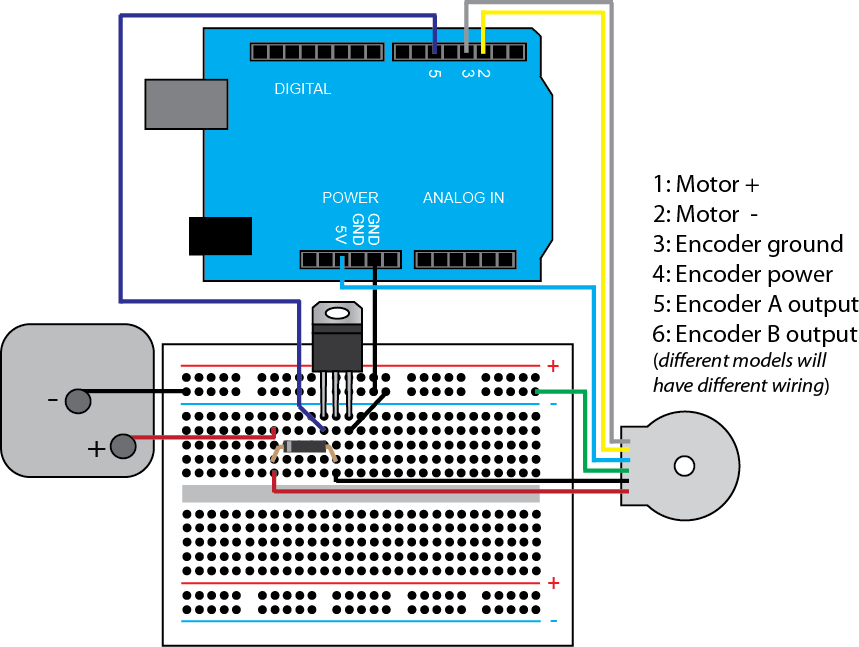
In the schematic shown, we employ a power MOSFET where the board drives the Gate pin. When voltage is supplied to the Gate, it closes the circuit between the Source and Drain pins. One possible choice of power MOSFET is the IRF1520 whose datasheet can be found here. For our diode, we will employ the general purpose 1N4007 whose datasheet can be found here.

We are able to achieve approximately continuous control of the motor's speed using only a DC source by employing Pulse-Width Modulation (PWM). Recall, a PWM approach alternately turns the motor "on" and "off". Since the motor has dynamics (inertia, friction, etc.), it doesn't instantaneously reach top speed when turned on and doesn't immediately come to a stop when turned off. It takes time for the motor to react. This can be used to our advantage if the PWM frequency is sufficiently fast. It's as if the motor is filtering the PWM command. In this way, the speed of the motor can be controlled continuously by varying the percent of time the PWM signal is on compared to the overall period (the duty cycle). Further details on PWM can be found in Activity 1b and Activity 4.

We will also employ the Arduino board for sensing the position/speed of the motor. There are different means for achieving this with one of the most popular being the optical encoder. An optical encoder consists of an emitter (a light source, like an LED) and a detector (a phototransistor). Within an encoder there is a piece of material that alternately blocks and passes light as the material is passed between the emitter/detector pair. When the phototransistor detects the light its output goes high, and when it doesn't detect light its output goes low. By counting these pulses, the sensor indicates the displacement of the material between the emitter and detector. Furthermore, by timing the frequency of these pulses, the sensor can be used to indicate speed.

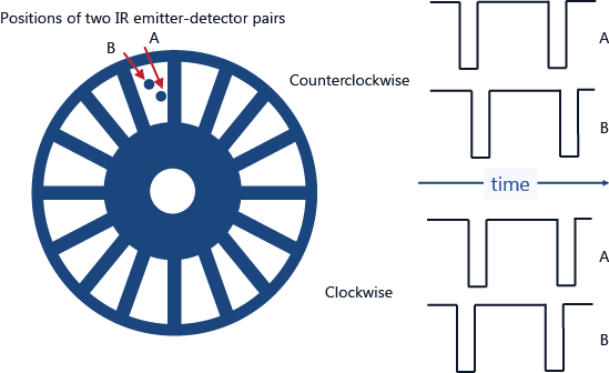
By employing two emitter/detector pairs that are slightly offset, the optical encoder can also be used to determine the direction of motion. In the following rotary example, when the disk is rotating counterclockwise the disk will encounter Pair A first and Pair B second, thereby causing channel A to go low before channel B goes low. When the disk is rotating clockwise, then channel B will go low first. This type of configuration is typical of what is referred to as quadrature.

Another commonly employed transducer is a Hall-effect sensor. A Hall-effect sensor is able to detect a magnetic field. By detecting the passing of gear teeth or a magnet, the Hall-effect sensor can generate a pulse-train output similar to that produced by an optical encoder. Furthermore, employing offset Hall-effect sensors can generate a quadrature output for determining the direction of motion.

One motor with Hall-effect encoder that could be used for this activity can be found here, though there are many other choices. This particular motor can be driven by a 6-V lantern type battery. The encoder provides 48 counts per revolution (if you count both rising and falling edges). The motor also includes a gearbox so that the Hall-effect sensor generates 1633 counts per revolution at the output shaft of the gearbox. A version of this motor can be purchased without the gearbox for less money here. Various accessories for the motor (brackets, wheels, etc.) can be found from the same website. The setup of the motor with encoder and its connection to the Arduino board is shown below. The color band on the diode indicates its cathode. The Gate, Source, and Drain pins of the MOSFET can be deduced from its orientation in the given figure.

Software setup

In this experiment, we will employ Simulink to control the motor through the switching of the transistor, to read the encoder output, and to plot the data in real time. In particular, we will employ the IO package from the MathWorks. For details on how to use the IO package, refer to the following link. We will build the Simulink model for this activity in a step-by-step manner in order to explain the nuances of using quadrature encoder output for sensing the motor's speed.

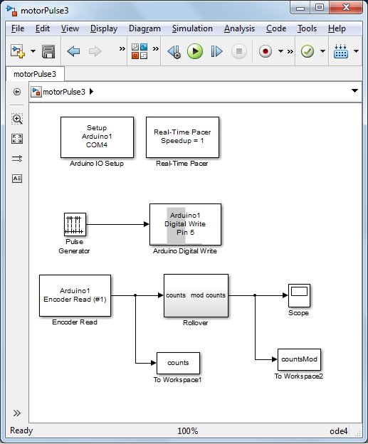
To begin, we will construct a model as shown below where you may need to change the port to which the Arduino board is connected (the port is COM4 in this case). The Pulse Generator block toggles between 0 and 1 and is connected to the Digital Write Block to switch the transistor between its OFF state and its ON state, respectively. Double-clicking the Pulse Generator block we set the Sample time equal to "0.02". In the downloadable model, the sample time is set to the variable Ts which needs to be defined in the MATLAB workspace by typing Ts = 0.02 before the model can be run. We will also define the Pulse type to be Sample based with a Period of "28/Ts" samples (28 seconds) and a Pulse width of "26/Ts" samples (26 seconds) and a Phase delay of "2/Ts" samples (2 seconds).

As the gate of the MOSFET is triggered from Digital Output 5, the Digital Write block needs to be set to the corresponding pin. Specifically, double-clicking on the block allows us to set the Pin to 5 from the drop-down menu. We will leave the Sample time as "-1" to inherit the value from the Pulse Generator block. The Encoder Read block is used for reading the quadrature encoder signal. The encoder pulses are counted via the program running on the Arduino board. The Encoder Read block polls the board every sample period to get the latest number of counts that have been accumulated. Double-clicking on the Encoder Read block, we will leave the Encoder Number as "1" (we only have one encoder so it doesn't matter). We will also set Pin A to "2" and Pin B to "3". These correspond to the pins to which we connected the quadrature encoder signals. For the Arduino Uno, this is the only option. For the Mega, for example, we could also use pins 18 and 19, or pins 20 and 21. The Sample time is again set to "0.02". Finally, we connect the output of the Encoder Read block to a Scope and a To Workspace block.

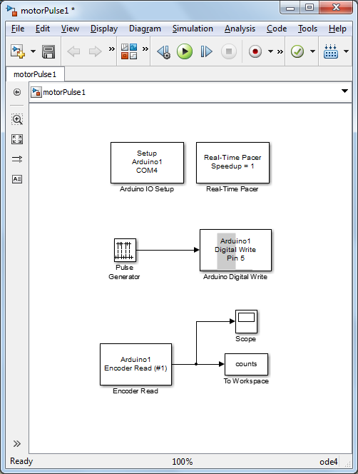
The Arduino Digital Write block, the Encoder Read block, the Arduino IO Setup block, and the Real-Time Pacer block are all part of the IO package. The remaining blocks are part of the standard Simulink library, specifically, they can be found under the Sources and Sinks libraries.

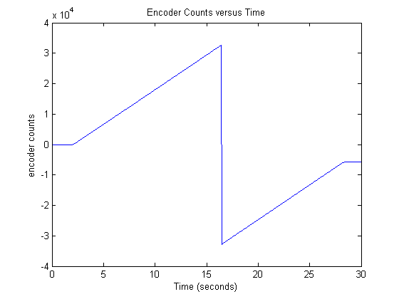
Running the above model for 30 seconds generates the figure shown below of encoder counts versus time. Examination of the figure shows that motor is initially at rest (number of counts aren't changing), then after 2 seconds the motor is turned on (the transistor is switched on) and the number of encoder counts increments as the motor spins. If the motor was spinning in the opposite direction, the encoder counts would decrement. Notice that around an elapsed time of 16 seconds, the number of encoder counts "rolls over." This happens because the buffer that is keeping track of the number of counts can only represent numbers between -32768 and 32767 (i.e. it uses 16-bits, 15 bits for the number and 1 bit for the sign).

Since we ultimately wish to estimate the motor's speed based on these counts, we somehow need to address this rollover. Specifically, we will construct the subsystem "Rollover" shown in the model below.

This subsystem compares the current number of counts to the number of counts from the previous sample in order to determine whether a rollover has occurred (at 32767 or at -32768) and then modifies the accumulated number of counts to remove the rollover. Looking within the rollover subsystem, shown below, you can inspect the logic used for correcting the accumulated number of counts.

If we re-run our Simulink model with the rollover correction, we now get the following response of encoder counts as a function of time.

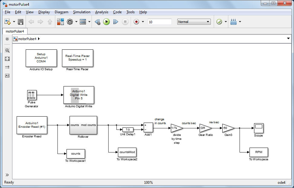
Next we wish to estimate the motor's speed based on the encoder counts by adding the following elements to our Simulink model. Since the encoder counts indicate the motor's position, we can approximate the motor's speed over a specific interval of time as the change in the motor's position divided by the change in time between samples. In essence, this is the motor's average speed over that time interval. Specifically, the Difference block computes the motor's change in position (in counts) and the first Gain block divides by the sample time. Subsequent Gain blocks convert the units from counts/sec to revolutions/sec, and then from revolutions/sec to revolutions/min. The constant representing the gear ratio needs to be defined in the MATLAB workspace before the model can be run. For the motor described above, we would type GR = 1/1633; at the command line.

Reducing the length of the simulation then running the model generates the following output for motor speed in RPM.

Examining the above, we can see that the estimate for motor speed is quite noisy. This arises for several reasons: the speed of the motor is actually varying, encoder counts are being periodically missed, the timing at which the board is polled doesn't exactly match the prescribed sampling time, and there is quantization associated with reading the encoder. In order to reduce the effect of noise, we can increase the sampling period and can add a filter to "smooth" the motor speed estimate. Consider the following model with a simple first-order filter added to the motor speed estimate. This model can be downloaded here.

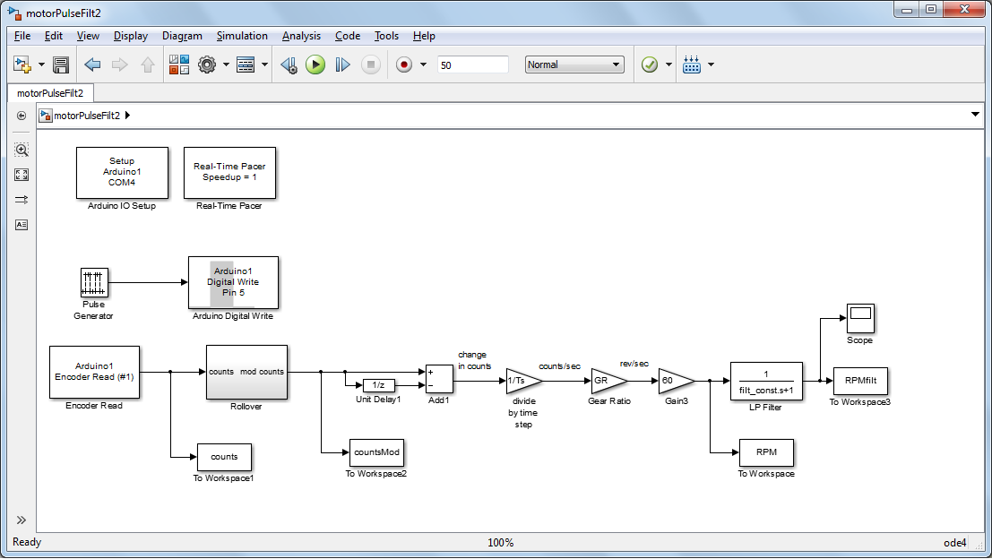
Running this model with the sample time increased to 0.05 seconds and a filter time constant of 0.15 seconds produces the following time trace for the motor speed. Make sure to define the necessary variables at the command line before running the model, Ts = 0.05; filter_constant = 0.15;.

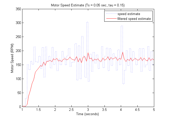
By increasing the sampling period and adding the filter, the speed estimate indeed is much less noisy. This is especially helpful for improving the estimate of the motor's speed when it is running at a steady speed. A drawback of the filtering, however, is that it adds delay. This can be seen by looking at the estimate with and without filtering at the point at which the input is "turned on." The filtered output lags behind the unfiltered input. In essence we have lost information about the motor's actual response. In this case, this makes identifying a model for the motor more challenging. In the case of feedback control, this lag can degrade the performance of the closed-loop system. Reducing the time constant of the filter will reduce this lag, but the tradeoff is that the noise won't be filtered as well.

In this activity we are attempting to infer a model for the motor based on its observed response. Considering that our input is a 6-Volt step, the observed response appears to have the form of a first-order step response. Looking at the filtered speed, the DC gain for the system is then approximately 170 RPM/ 6 Volts 28 RPM/V. In order to estimate the time constant, however, we need reduce the filtering in order to better see the true speed of the motor. Looking at the unfiltered data, and reducing the sample time to 0.01 seconds, we get the following speed response.

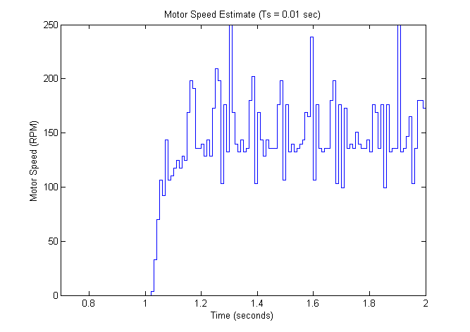
Recalling that a time constant defines the time it takes a process to achieve 63.2% of its total change, we can estimate the time constant from the above graph. We will attempt to "eye-ball" a fitted line to the motor's response graph. This too is like adding a filter, but since it doesn't have to occur in real-time, we can use future data (as well as past data) to avoid the introduction of lag. Assuming the same steady-state performance observed in the more heavily filtered data, we can estimate the time constant based on the time it takes the motor speed to reach RPM. Since this appears to occur at 1.06 seconds and the input appears to step at 1.02 seconds, we can estimate the motor's time constant to be approximately 0.04 seconds. Therefore, our blackbox model for the motor is the following.

(2)

Recalling the model of the motor we derived from first principles, repeated below. We can see that we anticipated a second-order model, but the response looks more like a first-order model. The explanation is that the motor is overdamped (poles are real) and that one of the poles dominates the response. This is typical of a DC motor where the mechanical dynamics are much slower than the electrical dynamics, and hence dominate the response.

(3)

In addition to the fact that our model is reduced-order, the model is a further approximation of the real world in that it neglects nonlinear aspects of the true physical motor. Based on our linear model, the motor's output should scale with inputs of different magnitudes. For example, the response of the motor to a 6-Volt step should have the same shape as its response to a 1-V step, just scaled by a factor of 6. In reality, however, if the applied voltage is sufficiently small, the motor won't move at all. This is due to the stiction in the motor. If the motor torque isn't large enough, the motor cannot "break free" of the stiction. This nonlinear behavior is not captured in our model. Typically, we use a viscous friction model that is linearly proportional to speed, rather than a Coulomb friction model that captures this stiction.

Extensions

Some extensions to this activity would be to try to identify the individual parameters of the motor. You could then compare the predictive ability of the physics-based model to the blackbox model. Another exercise would be to generate a blackbox model for the motor based on its frequency response, similar to what was done with the boost converter in Activity 5b. An advantage of using a frequency response approach to identification is that it enables identification of the non-dominant dynamics. In this case, however, those dynamics would need to be slower (or the measuring system faster) in order to identify them.

In Part (b) of this activity, we design a PI controller for the motor.

Published with MATLAB® 8.2