


Introduction: Digital Controller Design
In this section, we will discuss converting continuous-time models into discrete-time (or difference equation) models. We will also introduce the z-transform and show how to use it to analyze and design controllers for discrete-time systems.
Key MATLAB commands used in this tutorial are: c2d , pzmap , zgrid , step , rlocus
Contents
Introduction
The figure below shows the typical continuous-time feedback system that we have been considering so far in this tutorial. Almost all continuous-time controllers can be implemented employing analog electronics.

The continuous controller, enclosed in the shaded rectangle, can be replaced by a digital controller, shown below, that performs the same control task as the continuous controller. The basic difference between these controllers is that the digital system operates on discrete signals (samples of the sensed signals) rather than on continuous signals. Such a change may be necessary if we wish to implement our control algorithm in software on a digital computer, which is frequently the case.

The various signals of the above digital system schematic can be represented by the following plots.

The purpose of this Digital Control Tutorial is to demonstrate how to use MATLAB to work with discrete functions, either in transfer function or state-space form, to design digital control systems.
Zero-Hold Equivalence
In the above schematic of the digital control system, we see that the system contains both discrete and continuous portions. Typically, the system being controlled is in the physical world and generates and responds to continuous-time signals, while the control algorithm may be implemented on a digital computer. When designing a digital control system, we first need to find the discrete equivalent of the continuous portion of the system.
For this technique, we will consider the following portion of the digital control system and rearrange as follows.


The clock connected to the D/A and A/D converters supplies a pulse every  seconds and each D/A and A/D sends a signal only when the pulse arrives. The purpose of having this pulse is to require that
 acts only on periodic input samples
  , and produces periodic outputs
  only at discrete intervals of time; thus, can be realized as a discrete function.
The philosophy of the design is the following. We want to find a discrete function so that for a piecewise constant input to the continuous system  , the sampled output of the continuous system equals the discrete output. Suppose the signal represents a sample of the input signal. There are techniques for taking this sample and for holding it to produce a continuous signal
  . The sketch below shows one example where the continuous signal is held constant at each sample over the interval
  to
to  . This operation of holding constant over the sample period is called a zero-order hold.

The held signal then is passed to  and the A/D produces the output that will be the same piecewise signal as if the discrete signal had been passed through to produce the discrete output .

Now we will redraw the schematic, replacing the continuous portion of the system with .

Now we can design a digital control system dealing with only discrete functions.
Note: There are certain cases where the discrete response does not match the continuous response generated by a hold circuit implemented in a digital control system. For further information, see the page Lagging Effect Associated with a Hold.
Conversion Using c2d
There is a MATLAB function c2d that converts a given continuous system (either in transfer function or state-space form) to a discrete system using the zero-order hold operation explained above. The basic syntax for this in MATLAB is sys_d = c2d(sys,Ts,'zoh')
The sampling time (Ts in sec/sample) should be smaller than 1/(30BW), where BW is the system's closed-loop bandwidth frequency.
Example: Mass-Spring-Damper
Transfer Function
Suppose you have the following continuous transfer function model:
(1)
Assuming the closed-loop bandwidth frequency is greater than 1 rad/sec, we will choose the sampling time (Ts) equal to 1/100 sec. Now, create a new m-file and enter the following commands.
m = 1;
b = 10;
k = 20;

s = tf('s');
sys = 1/(m*s^2+b*s+k);

Ts = 1/100;
sys_d = c2d(sys,Ts,'zoh')
sys_d =

  4.837e-05 z + 4.678e-05
  -----------------------
  z^2 - 1.903 z + 0.9048

Sample time: 0.01 seconds
Discrete-time transfer function.
State-Space
A continuous-time state-space model of this system is the following:
(2)![$$
\mathbf{\dot{x}} = \left[ \begin{array}{c} \dot{x} \\ \ddot{x} \end{array} \right] = \left[ \begin{array}{cc} 0 & 1 \\ -\frac{k}{m} & -\frac{b}{m} \end{array} \right] \left[ \begin{array}{c} x \\ \dot{x} \end{array} \right] + \left[ \begin{array}{c} 0 \\ \frac{1}{m} \end{array} \right] F(t)
$$](Content/Introduction/Control/Digital/html/Introduction_ControlDigital_eq07631781795552767559.png)
(3)![$$
y = \left[ \begin{array}{cc} 1 & 0 \end{array} \right] \left[
\begin{array}{c} x \\ \dot{x} \end{array} \right]
$$](Content/Introduction/Control/Digital/html/Introduction_ControlDigital_eq10186743209670445684.png)
All constants are the same as before. The following m-file converts the above continuous-time state-space model to a discrete-time state-space model.
A = [0       1;
    -k/m   -b/m];

B = [  0;
    1/m];

C = [1 0];

D = [0];

Ts = 1/100;

sys = ss(A,B,C,D);
sys_d = c2d(sys,Ts,'zoh')
sys_d =

  A =
             x1        x2
   x1     0.999  0.009513
   x2   -0.1903    0.9039

  B =
              u1
   x1  4.837e-05
   x2   0.009513

  C =
       x1  x2
   y1   1   0

  D =
       u1
   y1   0

Sample time: 0.01 seconds
Discrete-time state-space model.
From these matrices, the discrete state-space can be written as
(4)![$$
\left[ \begin{array}{c} x(k) \\ v(k) \end{array} \right] =
\left[ \begin{array}{cc} 0.9990 & 0.0095 \\ -0.1903 & 0.9039 \end{array} \right] \left[ \begin{array}{c} x(k-1) \\ v(k-1) \end{array} \right] +
\left[ \begin{array}{c} 0 \\ 0.0095 \end{array} \right] F(k-1)
$$](Content/Introduction/Control/Digital/html/Introduction_ControlDigital_eq03225988395097153418.png)
(5)![$$
y(k-1) = \left[ \begin{array}{cc} 1 & 0 \end{array} \right] \left[ \begin{array}{c} x(k-1) \\ v(k-1) \end{array} \right]
$$](Content/Introduction/Control/Digital/html/Introduction_ControlDigital_eq00265804575559411755.png)
Now we have the discrete-time state-space model.
Stability and Transient Response
For continuous systems, we know that certain behaviors result from different pole locations in the s-plane. For instance, a system is unstable when any pole is located to the right of the imaginary axis. For discrete systems, we can analyze the system behaviors from different pole locations in the z-plane. The characteristics in the z-plane can be related to those in the s-plane by the following expression.
(6)
- T = sampling time (sec/sample)
- s = location in the s-plane
- z = location in the z-plane
The figure below shows the mapping of lines of constant damping ratio ( ) and natural frequency (
 ) from the s-plane to the z-plane using the expression shown above.

You may have noticed that in the z-plane the stability boundary is no longer the imaginary axis, but rather is the circle of radius one centered at the origin, |z| = 1, referred to as the unit circle. A discrete system is stable when all poles are located inside the unit circle and unstable when any pole is located outside the circle.
For analyzing the transient response from pole locations in the z-plane, the following three equations used in continuous system designs are still applicable.
(7)
(8)
(9)
where,
- = damping ratio
- = natural frequency (rad/sec)
 = 1% settling time
 = 10-90% rise time
 = maximum overshoot
Important: The natural frequency () in the z-plane has units of rad/sample, but when you use the equations shown above, must be represented in units of rad/sec.
Suppose we have the following discrete transfer function
(10)
Create a new m-file and enter the following commands. Running this m-file in the command window gives you the following plot with the lines of constant damping ratio and natural frequency.
numDz = 1;
denDz = [1 -0.3 0.5];
sys = tf(numDz,denDz,-1); % the -1 indicates that the sample time is undetermined

pzmap(sys)
axis([-1 1 -1 1])
zgrid
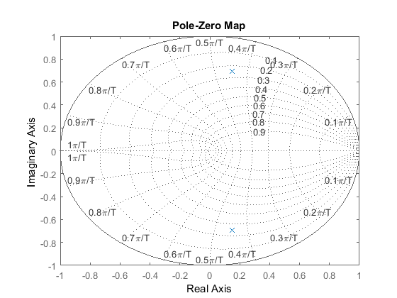
From this plot, we see the poles are located approximately at a natural frequency of  (rad/sample) and a damping ratio of 0.25. Assuming that we have a sampling time of 1/20 sec (which leads to = 28.2 rad/sec) and using the three equations shown above, we can determine that this system should have a rise time of 0.06
sec, a settling time of 0.65 sec, and a maximum percent overshoot of 45% (0.45 times more than the steady-state value). Let's
obtain the step response and see if these are correct. Add the following commands to the above m-file and rerun it in the
command window. You should obtain the following step response.
(rad/sample) and a damping ratio of 0.25. Assuming that we have a sampling time of 1/20 sec (which leads to = 28.2 rad/sec) and using the three equations shown above, we can determine that this system should have a rise time of 0.06
sec, a settling time of 0.65 sec, and a maximum percent overshoot of 45% (0.45 times more than the steady-state value). Let's
obtain the step response and see if these are correct. Add the following commands to the above m-file and rerun it in the
command window. You should obtain the following step response.
sys = tf(numDz,denDz,1/20);
step(sys,2.5);
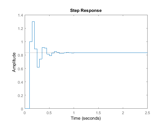
As we can see from the plot, the rise time, settling time and overshoot came out to be what we expected. This demonstrates how we can use the locations of poles and the above three equations to analyze the transient response of a discrete system.
Discrete Root Locus
The root-locus is the locus of points where roots of the characteristic equation can be found as a single parameter is varied
from zero to infinity. The characteristic equation of our unity-feedback system with simple proportional gain,  , is:
, is:
(11)
where  is the digital controller and is the plant transfer function in z-domain (obtained by implementing a zero-order hold).
The mechanics of drawing the root-loci are exactly the same in the z-plane as in the s-plane. Recall from the continuous Root-Locus Tutorial, we used the MATLAB function sgrid to find the root-locus region that gives an acceptable gain (). For the discrete root-locus analysis, we will use the function zgrid, which has the same function as sgrid. The syntax zgrid(zeta, Wn) draws lines of constant damping ratio (zeta) and natural frequency (Wn).
Suppose we have the following discrete transfer function
(12)
and the requirements are a damping ratio greater than 0.6 and a natural frequency greater than 0.4 rad/sample (these can be found from the design requirements, the sampling period (sec/sample), and the three equations shown in the previous section). The following commands draw the root-locus with the lines of constant damping ratio and natural frequency. Create a new m-file and enter the following commands. Running this m-file should generate the following root-locus plot.
numDz = [1 -0.3];
denDz = [1 -1.6 0.7];
sys = tf(numDz,denDz,-1);

rlocus(sys)
axis([-1 1 -1 1])

zeta = 0.4;
Wn = 0.3;
zgrid(zeta,Wn)
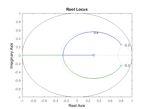
From this plot, we can see that the system is stable for some values of since there are portions of the root locus where both branches are located inside the unit circle. Also, we can observe two
dotted lines representing the constant damping ratio and natural frequency. The natural frequency is greater than 0.3 outside
the constant-Wn line, and the damping ratio is greater than 0.4 inside the constant-zeta line. In this example, portions of
the generated root-locus are within in the desired region. Therefore, a gain () chosen to place the two closed-loop poles on the loci within the desired region should provide us a response that satisfies
the given design requirements.
