Introduction: State-Space Methods for Controller Design

In this section, we will show how to design controllers and observers using state-space (or time-domain) methods.

Key MATLAB commands used in this tutorial are: eig , ss , lsim , place , acker

Modeling

There are several different ways to describe a system of linear differential equations. The state-space representation was introduced in the Introduction: System Modeling section. For a SISO LTI system, the state-space form is given below:

(1) $\frac{d\mathbf{x}}{dt} = A\mathbf{x} + Bu$

(2) $y = C\mathbf{x} + Du$

where $\mathbf{x}$ is an n by 1 vector representing the system's state variables, $u$ is a scalar representing the input, and $y$ is a scalar representing the output. The matrices $A$ (n by n), $B$ (n by 1), and $C$ (1 by n) determine the relationships between the state variables and the input and output. Note that there are n first-order differential equations. A state-space representation can also be used for systems with multiple inputs and multiple outputs (MIMO), but we will primarily focus on single-input, single-output (SISO) systems in these tutorials.

To introduce the state-space control design method, we will use the magnetically suspended ball as an example. The current through the coils induces a magnetic force which can balance the force of gravity and cause the ball (which is made of a magnetic material) to be suspended in mid-air. The modeling of this system has been established in many control text books (including Automatic Control Systems by B. C. Kuo, the seventh edition).

The equations for the system are given by:

(3) $m\frac{d^2h}{dt^2} = mg - \frac{Ki^2}{h}$

(4) $V = L\frac{di}{dt} + iR$

where $h$ is the vertical position of the ball, $i$ is the current through the electromagnet, $V$ is the applied voltage, $m$ is the mass of the ball, $g$ is the acceleration due to gravity, $L$ is the inductance, $R$ is the resistance, and $K$ is a coefficient that determines the magnetic force exerted on the ball. For simplicity, we will choose values $m$ = 0.05 kg, $K$ = 0.0001, $L$ = 0.01 H, $R$ = 1 Ohm, $g$ = 9.81 m/s^2. The system is at equilibrium (the ball is suspended in mid-air) whenever $h$ = $K i^2/mg$ (at which point $dh/dt$ = 0). We linearize the equations about the point $h$ = 0.01 m (where the nominal current is about 7 Amps) and obtain the linear state-space equations:

(5) $\frac{d\mathbf{x}}{dt} = A\mathbf{x} + Bu$

(6) $y = C\mathbf{x} + Du$

where:

(7) $x = \left[{\begin{array}{c} \Delta h \\ \Delta \dot{h} \\ \Delta i \end{array}}\right]$

is the set of state variables for the system (a 3x1 vector), $u$ is the deviation of the input voltage from its equilibrium value ( $\Delta V$ ), and $y$ (the output) is the deviation of the height of the ball from its equilibrium position ( $\Delta h$ ). Enter the system matrices into an m-file.

A = [ 0   1   0
     980  0  -2.8
      0   0  -100 ];

B = [ 0
      0
      100 ];

C = [ 1 0 0 ];

Stability

One of the first things we want to do is analyze whether the open-loop system (without any control) is stable. As discussed in the Introduction: System Analysis section, the eigenvalues of the system matrix, $A$ , (equal to the poles of the transfer function) determine stability. The eigenvalues of the $A$ matrix are the values of $s$ that are solutions of $\det(sI - A) = 0$ .

poles = eig(A)

poles =
   31.3050
  -31.3050
 -100.0000

From inspection, it can be seen that one of the poles is in the right-half plane (i.e. has positive real part), which means that the open-loop system is unstable.

To observe what happens to this unstable system when there is a non-zero initial condition, add the following lines to your m-file and run it again:

t = 0:0.01:2;
u = zeros(size(t));
x0 = [0.01 0 0];

sys = ss(A,B,C,0);

[y,t,x] = lsim(sys,u,t,x0);
plot(t,y)
title('Open-Loop Response to Non-Zero Initial Condition')
xlabel('Time (sec)')
ylabel('Ball Position (m)')

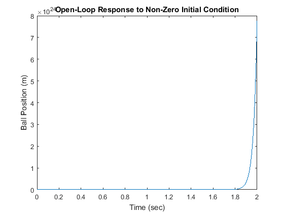
It looks like the distance between the ball and the electromagnet will go to infinity, but probably the ball hits the table or the floor first (and also probably goes out of the range where our linearization is valid).

Controllability and Observability

A system is controllable if there always exists a control input, $u(t)$ , that transfers any state of the system to any other state in finite time. It can be shown that an LTI system is controllable if and only if its controllabilty matrix, $\mathcal{C}$ , has full rank (i.e. if rank( $\mathcal{C}$ ) = n where n is the number of states variables). The rank of the controllability matrix of an LTI model can be determined in MATLAB using the commands rank(ctrb(A,B)) or rank(ctrb(sys)).

(8) $\mathcal{C} = [B\ AB\ A^2B\ \cdots \ A^{n-1}B]$

All of the state variables of a system may not be directly measurable, for instance, if the component is in an inaccessible location. In these cases it is necessary to estimate the values of the unknown internal state variables using only the available system outputs. A system is observable if the initial state, $x(t_0)$ , can be determined based on knowledge of the system input, $u(t)$ , and the system output, $y(t)$ , over some finite time interval $t_0 < t < t_f$ . For LTI systems, the system is observable if and only if the observability matrix, $\mathcal{O}$ , has full rank (i.e. if rank( $\mathcal{O}$ ) = n where n is the number of state variables). The observability of an LTI model can be determined in MATLAB using the command rank(obsv(A,C)) or rank(obsv(sys)).

(9) $\mathcal{O} = \left[ \begin{array}{c} C \\ CA \\ CA^2 \\ \vdots \\ CA^{n-1} \end{array} \right]$

Controllability and observability are dual concepts. A system ( $A$ , $B$ ) is controllable if and only if a system ( $A'$ , $B'$ ) is observable. This fact will be useful when designing an observer, as we shall see below.

Control Design Using Pole Placement

Let's build a controller for this system using a pole placement approach. The schematic of a full-state feedback system is shown below. By full-state, we mean that all state variables are known to the controller at all times. For this system, we would need a sensor measuring the ball's position, another measuring the ball's velocity, and a third measuring the current in the electromagnet.

For simplicity, let's assume the reference is zero, $r$ = 0. The input is then

(10) $u = -K\mathbf{x}$

The state-space equations for the closed-loop feedback system are, therefore,

(11) $\dot{\mathbf{x}} = A\mathbf{x} + B(-K\mathbf{x}) = (A-BK)\mathbf{x}$

(12) $y = C\mathbf{x}$

The stability and time-domain performance of the closed-loop feedback system are determined primarily by the location of the eigenvalues of the matrix ( $A-BK$ ), which are equal to the closed-loop poles. Since the matrices $A$ and $BK$ are both 3x3, there will be 3 poles for the system. By choosing an appropriate state-feedback gain matrix $K$ , we can place these closed-loop poles anywhere we'd like (because the system is controllable). We can use the MATLAB function place to find the state-feedback gain, $K$ , which will provide the desired closed-loop poles.

Before attempting this method, we have to decide where we want to place the closed-loop poles. Suppose the criteria for the controller were settling time < 0.5 sec and overshoot < 5%, then we might try to place the two dominant poles at -10 +/- 10i (at $\zeta$ = 0.7 or 45 degrees with $\sigma$ = 10 > 4.6*2). The third pole we might place at -50 to start (so that it is sufficiently fast that it won't have much effect on the response), and we can change it later depending on what closed-loop behavior results. Remove the lsim command from your m-file and everything after it, then add the following lines to your m-file:

p1 = -10 + 10i;
p2 = -10 - 10i;
p3 = -50;

K = place(A,B,[p1 p2 p3]);
sys_cl = ss(A-B*K,B,C,0);

lsim(sys_cl,u,t,x0);
xlabel('Time (sec)')
ylabel('Ball Position (m)')

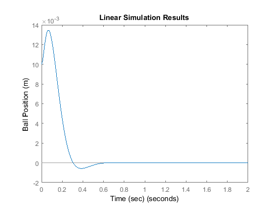
From inspection, we can see the overshoot is too large (there are also zeros in the transfer function which can increase the overshoot; you do not explicitly see the zeros in the state-space formulation). Try placing the poles further to the left to see if the transient response improves (this should also make the response faster).

p1 = -20 + 20i;
p2 = -20 - 20i;
p3 = -100;

K = place(A,B,[p1 p2 p3]);
sys_cl = ss(A-B*K,B,C,0);

lsim(sys_cl,u,t,x0);
xlabel('Time (sec)')
ylabel('Ball Position (m)')

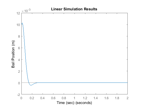
This time the overshoot is smaller. Consult your textbook for further suggestions on choosing the desired closed-loop poles.

Compare the control effort required ( $u$ ) in both cases. In general, the farther you move the poles to the left, the more control effort is required.

Note: If you want to place two or more poles at the same position, place will not work. You can use a function called acker which achieves the same goal (but can be less numerically well-conditioned):

K = acker(A,B,[p1 p2 p3])

Introducing the Reference Input

Now, we will take the control system as defined above and apply a step input (we choose a small value for the step, so we remain in the region where our linearization is valid). Replace t, u , and lsim in your m-file with the following:

t = 0:0.01:2;
u = 0.001*ones(size(t));

sys_cl = ss(A-B*K,B,C,0);

lsim(sys_cl,u,t);
xlabel('Time (sec)')
ylabel('Ball Position (m)')
axis([0 2 -4E-6 0])

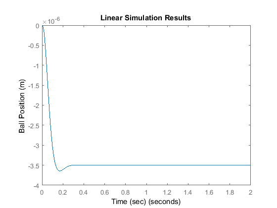
The system does not track the step well at all; not only is the magnitude not one, but it is negative instead of positive!

Recall the schematic above, we don't compare the output to the reference; instead we measure all the states, multiply by the gain vector $K$ , and then subtract this result from the reference. There is no reason to expect that $K\mathbf{x}$ will be equal to the desired output. To eliminate this problem, we can scale the reference input to make it equal to $K\mathbf{x}$ in steady-state. The scale factor, $\overline{N}$ , is shown in the following schematic:

We can calcuate $\overline{N}$ within MATLAB employing the function rscale (place the following line of code after K = ...).

Nbar = rscale(sys,K)

Nbar =
 -285.7143

Note that this function is not standard in MATLAB. You will need to download it here, rscale.m, and save it to your current workspace. Now, if we want to find the response of the system under state feedback with this scaling of the reference, we simply note the fact that the input is multiplied by this new factor, $\overline{N}$ :

lsim(sys_cl,Nbar*u,t)
title('Linear Simulation Results (with Nbar)')
xlabel('Time (sec)')
ylabel('Ball Position (m)')
axis([0 2 0 1.2*10^-3])

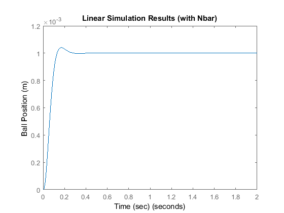
and now a step can be tracked reasonably well. Note, our calculation of the scaling factor requires good knowledge of the system. If our model is in error, then we will scale the input an incorrect amount. An alternative, similar to what was introduced with PID control, is to add a state variable for the integral of the output error. This has the effect of adding an integral term to our controller which is known to reduce steady-state error.

Observer Design

When we can't measure all state variables $\mathbf{x}$ (often the case in practice), we can build an observer to estimate them, while measuring only the output $y = C\mathbf{x}$ . For the magnetic ball example, we will add three new, estimated state variables ( $\hat{\mathbf{x}}$ ) to the system. The schematic is as follows:

The observer is basically a copy of the plant; it has the same input and almost the same differential equation. An extra term compares the actual measured output $y$ to the estimated output $\hat{y} = C\hat{\mathbf{x}}$ ; this will help to correct the estimated state $\hat{\mathbf{x}}$ and cause it to approach the values of the actual state $\mathbf{x}$ (if the measurement has minimal error).

(13) $\dot{\hat{\mathbf{x}}} = A\hat{\mathbf{x}} + Bu + L(y - \hat{y})$

(14) $\hat{y} = C\hat{\mathbf{x}}$

The error dynamics of the observer are given by the poles of $A-LC$ .

(15) $\dot{\mathbf{e}} = \dot{\mathbf{x}} - \dot{\hat{\mathbf{x}}} = (A - LC)\mathbf{e}$

First, we need to choose the observer gain $L$ . Since we want the dynamics of the observer to be much faster than the system itself, we need to place the poles at least five times farther to the left than the dominant poles of the system. If we want to use place, we need to put the three observer poles at different locations.

op1 = -100;
op2 = -101;
op3 = -102;

Because of the duality between controllability and observability, we can use the same technique used to find the control matrix by replacing the matrix $B$ by the matrix $C$ and taking the transposes of each matrix:

L = place(A',C',[op1 op2 op3])';

The equations in the block diagram above are given for the estimate $\hat{\mathbf{x}}$ . It is conventional to write the combined equations for the system plus observer using the original state equations plus the estimation error: $\mathbf{e} = \mathbf{x} - \hat{\mathbf{x}}$ . We use the estimated state for feedback, $u = -K \hat{\mathbf{x}}$ , since not all state variables are necessarily measured. After a little bit of algebra (consult your textbook for more details), we arrive at the combined state and error equations for full-state feedback with an observer.

At = [ A-B*K             B*K
       zeros(size(A))    A-L*C ];

Bt = [    B*Nbar
       zeros(size(B)) ];

Ct = [ C    zeros(size(C)) ];

To see how the response to a non-zero initial condition with no reference input appears, add the following lines into your m-file. Here we will assume that the observer begins with an initial estimate equal to zero, such that the initial estimation error is equal to the initial state vector, $\mathbf{e} = \mathbf{x}$ .

sys = ss(At,Bt,Ct,0);
lsim(sys,zeros(size(t)),t,[x0 x0]);

title('Linear Simulation Results (with observer)')
xlabel('Time (sec)')
ylabel('Ball Position (m)')

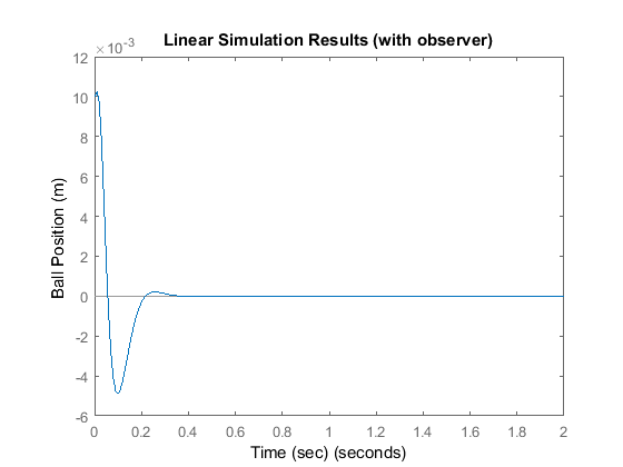
Responses of all the state variables are plotted below. Recall that lsim gives us $\mathbf{x}$ and $\mathbf{e}$ ; to get $\hat{\mathbf{x}}$ , we need to compute $\mathbf{x} - \mathbf{e}$ .

t = 0:1E-6:0.1;
x0 = [0.01 0.5 -5];
[y,t,x] = lsim(sys,zeros(size(t)),t,[x0 x0]);

n = 3;
e = x(:,n+1:end);
x = x(:,1:n);
x_est = x - e;

% Save state variables explicitly to aid in plotting
h = x(:,1); h_dot = x(:,2); i = x(:,3);
h_est = x_est(:,1); h_dot_est = x_est(:,2); i_est = x_est(:,3);

plot(t,h,'-r',t,h_est,':r',t,h_dot,'-b',t,h_dot_est,':b',t,i,'-g',t,i_est,':g')
legend('h','h_{est}','hdot','hdot_{est}','i','i_{est}')
xlabel('Time (sec)')

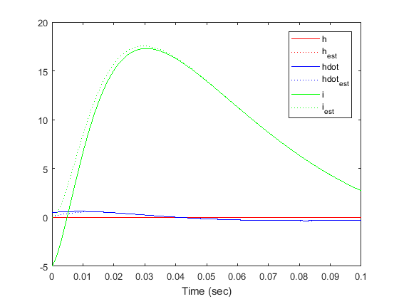
From the above, we can see that the observer estimates converge to the actual state variables quickly and track the state variables well in steady-state.