


Activity 1 Part (a): Time-Response Identification of a Resistor–Capacitor (RC) Circuit

Key Topics: Modeling Electrical Systems, First-Order Systems, System Identification
Contents
Equipment needed
- Arduino board (e.g. Uno, Mega 2560, etc.)
- USB cable
- Breadboard
- Electronic components (resistor and capacitor)
- Ohmmeter, Capacitance meter (optional)
- Jumper wires
The system we will be employing in this activity is a simple electrical circuit consisting of a resistor (R) and a capacitor (C) in series. The Arduino board will be used for generating the input to this RC circuit and for measuring the output of the circuit. Specifically, the input to the circuit will be a 5-Volt step, generated from one of the board's Digital Outputs, applied across the resistor and capacitor. The output of the circuit will be the voltage across the capacitor which will be read via one of the board's Analog Inputs. This data is then fed to Simulink for visualization and for comparison to our resulting simulation model output.
Purpose
The purpose of this activity is to demonstrate how to model a simple electrical system. Specifically, a first principles approach based on the underlying physics of the circuit and a blackbox approach based on recorded data will be employed. The associated experiment is employed to demonstrate the blackbox approach, as well as to demonstrate the accuracy of the resulting models. This activity also provides a physical example of the common class of first-order systems.
Modeling from first principles
First we will employ our understanding of the underlying physics of the RC circuit to derive the structure of the system model. We will term this process "modeling from first principles." In this example we employ the following variables.
(R) resistance of the resistor
(C) capacitance of the capacitor
(ei) input voltage
(eo) output voltage

To begin, we assume a direction for the current and then apply Kirchhoff’s Voltage Law (loop law). Current flows from a higher potential to a lower potential, therefore, the direction of the current will be clockwise in this case (shown below).

The loop law states that the sum of voltages around a closed loop must equal zero. Thus, the loop law produces the following governing equation for the circuit.
(1)
An alternative to the intregro-differential equation model of a dynamic system is the transfer function. The transfer function captures the input/output behavior of a system and is derived by first taking the Laplace transform
of a given integro-differential equation, while assuming zero initial conditions ( ).
).
(2)
Next we must perform some algebra to re-arrange the above into the form of its output divided by its input. In this case,
our input is  and our output is
  . Therefore, we must eliminate the current
  from the above since it is neither an input nor an output, and we must introduce the output into the above equation. Solving the above equation for we arrive at the following.
(3)
Then we can recognize that the output voltage (across the capacitor) is 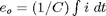 . Taking the Laplace transform and again solving for , we arrive at the following.
(4)
Setting the two previous equations equal to one another, we can eliminate .
(5)
Then re-arranging into the desired form of output divided by input, we produce the resulting transfer function model.
(6)
Recognizing the above as a first-order system, we can manipulate the transfer function so that it has the standard form shown below.
(7)
In this form we can see by inspection how the parameters of the circuit affect its response. Specifically, the values of the
resistor and capacitor affect the circuit's speed of response as indicated by their influence on the circuit's time constant,
 . The circuit components, however, cannot influence the circuit's steady-state performance as indicated by the fact that the
DC gain
. The circuit components, however, cannot influence the circuit's steady-state performance as indicated by the fact that the
DC gain  always equals 1.
System identification experiment
In this experiment we will record the output voltage of the RC circuit for a step in input voltage. Based on the resulting time response of the output voltage, we will fit a model to the data. This approach is sometimes referred to as blackbox modeling or data-driven modeling. After we have generated such a model, we will compare it to the first-principles derived model we created previously.
Hardware setup
Our simple RC circuit can be implemented on a breadboard and connected to the Arduino board as shown. One thing to note is that if you employ an electrolytic capacitor, its orientation matters. Specifically, if your capacitor has legs of different lengths and one leg is marked by a negative sign, then you have an electrolytic capacitor. Orient an electrolytic capacitor so that the leg marked by the negative sign connects to the lower potential part of the circuit (ground in this case). The Arduino board is employed to receive the input command from Simulink and to apply the input voltage to the circuit (via a Digital Output). The board also acquires the output voltage data from the circuit (via an Analog Input) and communicates the data to Simulink.

In this experiment, the values of the resistor and capacitor are chosen such that the circuit's time response is slow enough
that the Arduino/Simulink setup can sample the circuit at a fast enough rate to give a clear picture of the circuit's output.
If the sampling rate is at least 10 times faster than the circuit's time constant, we will be able to get a clear picture
of the response. In this experiment, we chose  and
and  to produce a circuit with time constant
  second. This is a low power application so most resistors and capacitors available will work fine, just make sure that the
capacitor is rated for at least 5 Volts.
second. This is a low power application so most resistors and capacitors available will work fine, just make sure that the
capacitor is rated for at least 5 Volts.
Software setup
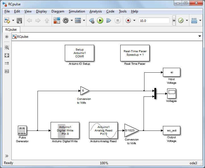
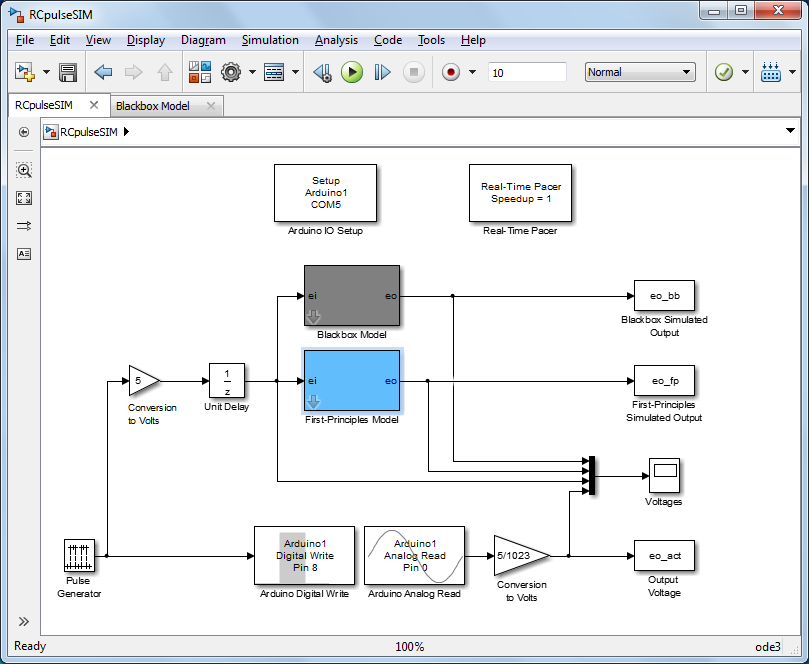
In this experiment, we will employ Simulink to read the data from the board and to plot the data in real time. In particular, we will employ the IO package from the MathWorks. For details on how to use the IO package, refer to the following link. The Simulink model we will use is shown below and can be downloaded here, where you may need to change the port to which the Arduino board is connected (the port is COM5 in this case).
As shown below, the input voltage command is generated by a Pulse Generator block. This block is chosen because of its generality, though for this experiment we could have used a Step block. The Pulse Generator block generates values of 0 or 1 which are then fed to an Arduino Digital Write block. Since we are using channel 8 for the digital output, we double-click on the Arduino Digital Write block to set the Pin to 8 from the drop-down menu. An input of 0 to the Digital Write block causes an output of 0 Volts to be generated at the corresponding pin, while an input of 1 to the Digital Write block generates an output of 5 Volts. This scaling is captured by the Gain block that is included prior to the Scope block. In this model the Pulse Generator block is set to output 0 for the first 5 seconds of the run in order to discharge the capacitor completely (in case it had built up charge) before stepping to 1 for the last 5 seconds of the run.
The Arduino Analog Read block reads the output voltage data via the Analog Input A0 on the board. Double-clicking on the block
allows us to set the Pin to 0 from the drop-down menu. We also will set the Sample Time to "0.1". This is 10 times faster than the circuit's time constant and hence is sufficiently fast. The other blocks in the
model can also be set to have a Sample Time of "0.1" (or left as "-1"). In the downloadable model, the sample time is set to the variable Ts which needs to be defined in the MATLAB workspace by typing Ts = 0.1 before the model can be run. The Gain block on the Analog Input is included to convert the data into units of Volts (by multiplying
the data by 5/1023). This conversion can be understood by recognizing that the Arduino Board employs a 10-bit analog-to-digital
converter, which means (for the default) that an Analog Input channel reads a voltage between 0 and 5 V and slices that range
into  pieces. Therefore, 0 corresponds to 0 V and 1023 corresponds to 5 V.
The given Simulink model then plots the commanded input voltage and recorded output voltage on a scope and also writes the output data, as an array, to the MATLAB workspace for further analysis. The Arduino Digital Write block, the Arduino Analog Read block, the Arduino IO Setup block, and the Real-Time Pacer block are all part of the IO package. The remaining blocks are part of the standard Simulink library, specifically, they can be found under the Math, Sources, and Sinks libraries.
Once the Simulink model has been created, it can then be run to collect the input voltage and output voltage data. Executing the following code at the MATLAB command line will generate the graph shown below. Note that we plot only the last five seconds of the run, thereby excluding any discharging of the capacitor that may have taken place.
         plot(0:0.1:5,ei(51:101),'r--');
         hold on
         plot(0:0.1:5,eo_act(51:101),'b*-');
         xlabel('time (seconds)')
         ylabel('voltage (Volts)')
         title('RC Circuit Step Response')
         legend('input','experimental output','Location','SouthEast')
         axis([0 5 0 5.1])

Parameter identification
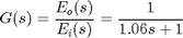
Based on the on the above figure, we can fit a model to the recorded data. Recognizing that the observed data has the shape of a first-order step response, we will assume the following standard first-order model for the circuit (happens to match our first-principles model).
(8)
We can then identify the system parameters and  from the recorded response data. Specifically, the steady-state value of the response indicates that the DC gain is
  . Note, we verified with a Voltmeter that the output voltage generated via the Digital Output was very close to 5 Volts. Recalling
that by definition the time constant represents the time it takes the system's response to reach
. Note, we verified with a Voltmeter that the output voltage generated via the Digital Output was very close to 5 Volts. Recalling
that by definition the time constant represents the time it takes the system's response to reach  of its total change, can be calculated from the following where 63.2 percent of 5 is approximately 3.16.
         plot(0:0.1:5,eo_act(51:101),'b*-');
         xlabel('time (seconds)')
         ylabel('voltage (Volts)')
         title('RC Circuit Step Response')
         legend('experimental output','Location','SouthEast')
         axis([0 5 0 5])

Since the step input occurs at approximately 0.10 seconds and the output reaches 3.16 Volts at approximately 1.16 seconds,
the time constant can be identified as  seconds. In reality, we only have data at intervals of 0.1 seconds, but using a datatip in the MATLAB plot allows us to interpolate
between the samples. Using a smaller sample period would allow us to improve the accuracy of our identification of the system
parameters. In conclusion, our resulting blackbox model is the following.
seconds. In reality, we only have data at intervals of 0.1 seconds, but using a datatip in the MATLAB plot allows us to interpolate
between the samples. Using a smaller sample period would allow us to improve the accuracy of our identification of the system
parameters. In conclusion, our resulting blackbox model is the following.
(9)
Model validation - forced response
In the this section we will validate the two circuit models we have derived, the first-principles model and the blackbox model, by comparing the step responses predicted by the models to actual data recorded from the circuit.
Recall the model that we derived from first principles earlier.
(10)
We will generate a Simulink model of this governing equation by first solving the equation for its highest-order "derivative."
(11)
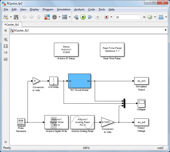
This equation is then represented in Simulink as shown below by the highlighted blocks (where R and C are variables). We have inserted these blocks into the existing Simulink model so that we may directly compare the simulated output voltage to the actual recorded output voltage. The Unit Delay block is added so that the timing of the simulated input voltage better matches the timing of the input voltage generated by the Arduino board. The To Workspace blocks are set to have Array outputs.

We could have also represented the first-principles model as a transfer function, but then we wouldn't be able to directly include initial conditions (an initial charge on the capacitor). The charge on the capacitor is the output of the Integrator block and its initial condition is set by double-clicking on the Integrator block. In the downloadable version of the model the initial condition is set to the variable "q_init" as shown below.

In order to make our Simulink model cleaner, we can create a subsystem for our first-principles model. Specifically, we can select the blocks highlighted in the above figure and then right-click. From the resulting menu we then choose Create Subsystem from Selection. We can also change the color of the block by choosing Format > Background Color > Light Blue from the resulting menu. Labeling the subsystem as "RC Circuit Model" gives us the Simulink model shown below.
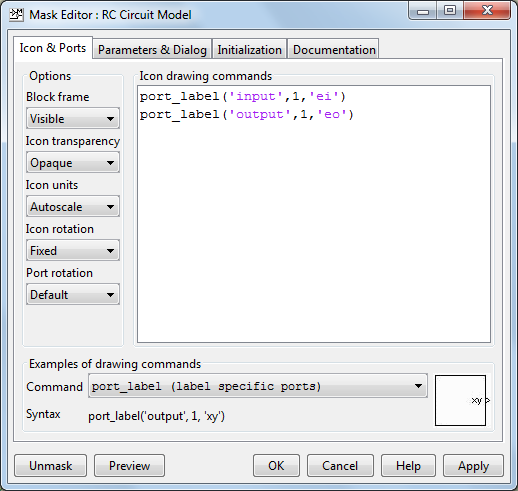
Going a step further, we can also create a mask for this subsystem by right-clicking on its block and selecting Mask > Create Mask... from the resulting menu. The creation of a mask for the subsystem allows us to specify the subsystem's parameters (R, C, and q_init) from within Simulink without delving into specific blocks. Specifically, right-click on the RC Circuit Model and select Mask > Edit Mask.... Under the panel Icon & Ports, type the following commands in the Icon drawing commands window as shown.
Next, click on panel Parameters & Dialog tab and select or drag the Edit icon in the left palette to add parameters to the Dialog box shown below. For the first parameter, enter "Resistance" under the Prompt column and "R" under the Name column. Repeat this process two more times for the "Capacitance" and the "Initial charge on capacitor" as shown below.

This window is then closed and the settings saved by clicking the OK button. If you double-click on RC Circuit Model again, you will find that the mask with desired parameters has been generated.
The values of R, C, and q_int are set to match the parameters of our physical system. For this experiment, recall that we are employing a  resistor, a
  capacitor, and we are observing the step response when when the capacitor is initially discharged.

Running this model, we can then compare the simulated output voltage eo_sim to the actual experimental output voltage eo_act. Recall that the Pulse Generator block is set to output 0 for the first 5 seconds of the run in order to discharge the capacitor completely before stepping to 1. Entering the following code in the MATLAB command window will generate the figure shown below.
         plot(0:0.1:5,eo_act(51:101),'b*-');
         hold on
         plot(0:0.1:5,eo_sim(51:101),'r--');
         xlabel('time (seconds)')
         ylabel('voltage (Volts)')
         title('RC Circuit Step Response')
         legend('experiment','model (first principles)','Location','SouthEast')

The above figure shows pretty good, though not exact, agreement between the output voltage predicted by our first-principles model and the physical circuit. We will discuss the accuracy of this model momentarily, but let's first investigate the performance of our blackbox model.
Recall that in the System identification experiment section we estimated the system parameters as  and
and  leading to the following blackbox model.
(12)
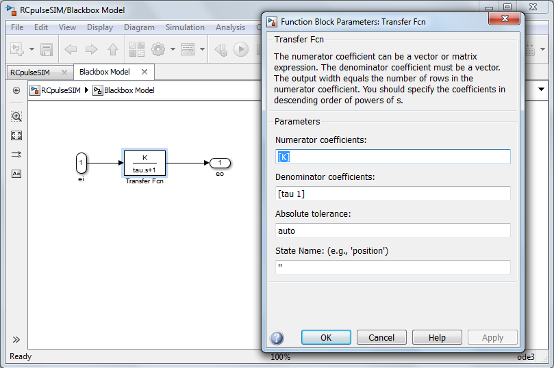
We can generate the blackbox model in Simulink using the Transfer Function block. Double-clicking on the Transfer Function block we can set Numerator coefficients equal to the variable "K" and the Denominator coefficients equal to "[tau 1]" where tau is also a variable, the time constant.
We can then create a subsystem with a mask for this blackbox model in the same manner we did for the first-principles model. The resulting Simulink model is shown below and can be downloaded here. Remember to set the parameters for the blackbox subsystem parameters K and tau.
Recall in the above that our first principles model did not exactly predict the output generated by the actual physical circuit. One factor contributing to this difference could be that the components (the resistor and capacitor) have actual values that differ from their nominal labels. We can improve our model by measuring the actual resistance and capacitance using an Ohmmeter and a capacitance meter, respectively.
In this experiment, the actual R is measured to be 9840  , compared with the label of
  , while the actual C is measured to be
  , compared with the label
  . Entering these values into the mask of our first principles model in Simulink, we can then re-run our simulation. Executing
the following MATLAB commands then generates the figure below showing the agreement between the two models and the experimental
data.
. Entering these values into the mask of our first principles model in Simulink, we can then re-run our simulation. Executing
the following MATLAB commands then generates the figure below showing the agreement between the two models and the experimental
data.
         plot(0:0.1:5,eo_act(51:101),'b*-');
         hold on
         plot(0:0.1:5,eo_fp(51:101),'r--');
         plot(0:0.1:5,eo_bb(51:101),'k--');
         xlabel('time (seconds)')
         ylabel('voltage (Volts)')
         title('RC Circuit Step Response')
         legend('experiment','model (first principles)','model (blackbox)','Location','SouthEast')

Examining the above, the blackbox model matches the data extremely well, while the addition of more accurate estimates of R and C did not improve the agreement with the first-principles model significantly. It is hypothesized that the error in the first principles model is likely due to the unmodeled resistance and capacitance of the input and output channels connected to the circuit. Such loading effects could be captured by the blackbox model since the true response appears to fit the form of a first-order model well.
It is generally the case that a blackbox model will be quite accurate when it is applied to the same situation (input, environmental conditions, etc.) from which it was derived. A blackbox model can, however, break down if it is applied under different conditions. This is in particular true if the model doesn't accurately capture the underlying structure of the system. We will, therefore, test our models under different conditions in the next section. In this case since we know that the structure of our first-principles model matches the structure of our blackbox model (both first order) and since the resistance and capacitance likely won't change much (at least over a short time period), our blackbox model should still perform well. A primary advantage of employing a blackbox model, aside from its accuracy, is that one does not need to understand the underlying system well in order to derive a model for it.
Model validation - free response
In the previous section we examined how well our models predicted the RC circuit's step response. That case examined the system's
response for a forcing input of a 5-Volt step in input voltage and zero initial conditions (no initial charge on the capacitor).
In this section we will investigate how well the models predict the RC circuit's free response. This case will assume no forcing
input,  , and an initial charge on the capacitor. This process will illustrate how to deal with initial conditions in our models.
To begin, we will solve for the theoretical free response we will expect from the RC circuit. Specifically, we will solve the governing equation we derived from first principles using the Laplace transform. This governing equation is repeated below.
(13)
The above is an integro-differential equation in terms of the current through the circuit  . We will re-write the above as a differential equation in terms of charge on the capacitor
  using the following definitions.
(14)
(15)
Therefore, the governing equation in terms of is the following.
(16)
Recalling that for this case , we can rearrange the differential equation as follows.
(17)
Then taking taking the Laplace transform.
(18)
Recalling that a capacitor's capacitance is defined as the amount of charge it can hold for a given potential difference,
 , we can express the initial charge on the capacitor in terms of the initial voltage across the capacitor (the initial output
voltage).
, we can express the initial charge on the capacitor in terms of the initial voltage across the capacitor (the initial output
voltage).
(19)
Substituting for  and solving the equation for
  gives the following.
(20)
Applying inverse Laplace transform, we then have the time response of the charge on the capacitor.
(21)
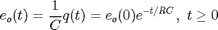
Again using the definition of capacitance, we then have the output response of the RC circuit for some initial charge and no forcing input voltage.
(22)
The above equation represents the theoretical free response expected from the RC circuit based on the first-principles model
we derived. We would like to compare the prediction of the first-principles model with that of the blackbox model and the
performance of the actual physical circuit. One challenge is that the blackbox model is in the form of a transfer function
which does not address initial conditions. This can be addressed by running the existing Simulink model from zero initial
conditions and then bringing the models and physical circuit to the desired initial state (level of capacitor charge). For
our existing Simulink model with Pulse Generator input, we could run the model for 15 seconds where for the first 5 seconds
the input is 0 to discharge the capacitor completely, for the next 5 seconds the input is 1 in order to charge the capacitor
completely ( Volts), and the final 5 seconds represents the free response as the input drops back to 0. You can change the simulation
run time in the toolbar of the window of your Simulink model, or via the drop-down menu Simulation > Model Configuration Parameters under the Solver menu. Running the existing model under these conditions and executing the following MATLAB commands will generate the figure
shown below.
Volts), and the final 5 seconds represents the free response as the input drops back to 0. You can change the simulation
run time in the toolbar of the window of your Simulink model, or via the drop-down menu Simulation > Model Configuration Parameters under the Solver menu. Running the existing model under these conditions and executing the following MATLAB commands will generate the figure
shown below.
         plot(0:0.1:5,eo_act(101:151),'b*-');
         hold on
         plot(0:0.1:5,eo_fp(101:151),'r--');
         plot(0:0.1:5,eo_bb(101:151),'k--');
         xlabel('time (seconds)')
         ylabel('voltage (Volts)')
         title('RC Circuit Free Response')
         legend('experiment','model (first principles)','model (blackbox)')

Examining the above, the blackbox model still provides better agreement with the recorded output voltage from the physical RC circuit than does the first-principles model. Recall that this difference is attributed to the fact that the first-principles model does not capture the effects of the input and output channel. The results from the blackbox model, however, do not seem to agree with the experimental data in this case as well as it did with the step response experiment. This difference is anticipated since the blackbox model was derived based on an identical step response experiment, rather than for the conditions of this free response experiment. That being said, the blackbox model still agrees with the physical data very well. This is attributable to the fact that the physical RC circuit is simple, approximately linear, and relatively time invariant.
As mentioned previously, the blackbox model is represented as a transfer function which does not explicitly allow the inclusion
of initial conditions. An alternative viewpoint for the blackbox model is to consider it as a linearization about some nominal
operating point of the true (nonlinear) physical system. In that manner the input and output can be considered as the deviation
of  and
and  from their initial conditions. That is
(23)
where  and
and  . Thinking of the blackbox model in this manner ensures that the initial conditions are always zero and hence can be modeled
by a transfer function. With this in mind, the blackbox model can be represented in Simulink in the following manner.
. Thinking of the blackbox model in this manner ensures that the initial conditions are always zero and hence can be modeled
by a transfer function. With this in mind, the blackbox model can be represented in Simulink in the following manner.

Extensions
An interesting change that can be made to this experiment is to replace the fixed resistor with a variable resistor (a trimmer potentiometer) to observe directly how the circuit's response changes with resistance. This can also be done with a variable capacitor, or by even swapping the resistor and capacitor with fixed components of different values.
In Part (b) of this activity, the frequency response characteristics of the RC circuit are investigated.
