Activity 2 Part (b): Electrical Circuits in Series

Key Topics: Modeling Electrical Systems, Loading, Higher-Order Systems, Filtering, Isolation

Equipment needed
Purpose
Modeling without loading
Hardware experiment
Modeling with loading
Adding an isolating amplifier

Equipment needed

Arduino board (e.g. Uno, Mega 2560, etc.)
Breadboard
Battery (AA for example)
Electronic components (inductor, resistors, capacitors)
Switch (pushbutton, or can employ a transistor)
Jumper wires

In this activity, we will examine the previously considered LRC circuit. Specifically, we will examine the LRC circuit when placed in series with an RC circuit of the form examined in Activity 1a. The hardware and software employed will largely be the same as used in the original LRC circuit activity. The input to the circuit will be a voltage step, supplied by a battery via a push-button switch. The output of the circuit will be the voltage across the capacitor of the RC circuit which will be read via one of the Arduino board's Analog Inputs. This data is then fed to Simulink for visualization.

Purpose

The purpose of this activity is to demonstrate how to model circuits in series. In particular, the phenomenon of loading is investigated. Also, how to predict the response of higher-order systems is discussed.

Modeling without loading

In this activity we will examine an LRC circuit in series with an RC circuit. We will use a subscript "1" for the components in the LRC circuit and a subscript "2" for the components in the RC circuit.

(R1)         resistance of the resistor in the LRC circuit

(R2)         resistance of the resistor in the RC circuit

(L)          inductance of the inductor

(Req)        equivalent series resistance (ESR) of the inductor

(C1)         capacitance of the capacitor in the LRC circuit

(C2)         capacitance of the capacitor in the RC circuit

(ei)         input voltage

(eo)         output voltage

Recalling the results of the model derivation in previous activities, we generated the following transfer function models for the LRC circuit and the RC circuit when considered separately. Here we introduce an intermediate variable $e'$ representing the voltage drop across the capacitor of the LRC circuit.

(1) $G_{LRC}(s) = \frac{E'(s)}{E_i(s)} = \frac{1}{LC_1s^2 + (R_1 + R_{eq})C_1s + 1}$

(2) $G_{RC}(s) = \frac{E_o(s)}{E'(s)} = \frac{1}{R_2C_2s + 1}$

When modeled as transfer functions, one generally combines systems in series by multiplying their transfer functions.

(3) $G_{series} = \frac{E_o(s)}{E_i(s)} = \frac{E'(s)}{E_i(s)}\cdot\frac{E_o(s)}{E'(s)} = \frac{1}{(LC_1s^2 + (R_1 + R_{eq})C_1s + 1)(R_2C_2s + 1)}$

(4) $\Rightarrow G_{series} = \frac{1}{LR_2C_1C_2s^3 + ((R_1 + R_{eq})R_2C_1C_2 + LC_1)s^2 + ((R_1 + R_{eq})C_1 + R_2C_2)s + 1}$

In the case of circuits, we cannot in general combine subsystems in this manner because the downstream circuit will load the upstream circuit. For example, when the LRC circuit is considered on its own there is only a single path for the current to flow through; the current through the resistor and inductor is the same as the current through the capacitor. When the RC circuit is placed in series with the LRC circuit, some of the current is diverted away from the path with $C_1$ and through the path with $R_2$ and $C_2$ . The addition of the downstream circuit affects the behavior of the upstream circuit. If the downstream circuit is high impedance, such that it does not draw much current away from the upstream circuit, then we can effectively neglect the loading and can consider the circuits independently. This is why it is desired for any measurement channel to have high impedance, so that it does load the circuit that is being measured. One can imagine such loading effects in other types of systems that involve flow, such as with fluid systems.

In the next section we will perform an experiment to determine if the loading effect is significant.

Hardware experiment

In this experiment we will record the output voltage of the series circuit for a step in input voltage. We then will compare the data to the response predicted by the previously derived model where we neglected the effect of loading. We will attempt to determine the conditions under which the loading effect becomes significant. The hardware and software setup we will employ is similar to what was employed for Part (a) of this experiment where the LRC circuit was considered on its own.

Hardware setup

The simple series circuit can be implemented on a breadboard and will employ a battery as the voltage source with a push-button switch. The act of completing the circuit with the switch will generate the step input to the circuit, while the voltage output will be read via an Analog Input of the Arduino board.

The setup of the series circuit and its connection to the Arduino board is shown below. Throughout the experiment we will employ the same LRC circuit that we employed in Part (a) of this activity ( $R_1 = 10 \Omega$ , $L = 1\ H$ , $R_{eq} = 40 \Omega$ , $C_1 = 510\ \mu F$ ). For the RC circuit, we will begin with the size of components employed in Activity 1 ( $R_2 = 10\ k\Omega$ , $C_2 = 100\ \mu F$ ), but as we progress we will alter the component sizes to better understand the loading effect.

Software setup

In this experiment, we will employ Simulink to read the data from the board and to plot the data in real time. In particular, we will employ the IO package from the MathWorks. For details on how to use the IO package, refer to the following link. We will use the same Simulink model employed in Part (a) of this activity. It is shown below and can be downloaded here, where you may need to change the port to which the Arduino board is connected (the port is COM3 in this case).

As shown below, this Simulink model simply reads the output voltage of the series circuit. Specifically, the Arduino Analog Read block reads the output voltage data via the Analog Input A0 on the board. Double-clicking on the block allows us to set the Pin to 0 from the drop-down menu. We also will set the Sample Time. We will maintain the sampling time we employed while examining the LRC circuit by itself, 0.01 seconds, though the addition of the slow RC circuit dynamics would allow a larger sample time. The downloadable model included above defines all sample times as Ts (or left as "-1"). Therefore, before you run this model you must define the variable Ts in the MATLAB workspace by typing Ts = 0.01; at the command line.

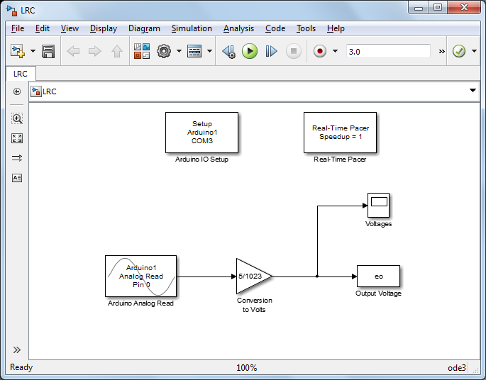
The other blocks in the model can also be set to have a sample time of Ts. The Gain block is included to convert the data into units of Volts (by multiplying the data by 5/1023). The given Simulink model then plots the recorded output voltage on a scope and also writes the output data to the MATLAB workspace for further analysis. The Arduino Analog Read block, the Arduino IO Setup block, and the Real-Time Pacer block are all part of the IO package. The remaining blocks are part of the standard Simulink library, specifically, they can be found under the Math and Sinks libraries.

Recall that the "step input" to our circuit is generated employing a push button as described earlier. Therefore, once you begin the model running, you will need to press the push button to cause the input voltage to step. One such set of data is shown below. Note that this data is for the case that the capacitors initially have no charge. If you are performing successive runs and wish to begin with an initial output voltage of zero, then you will need to discharge the capacitors before performing a run. This can be done by simply shorting (placing a wire between) the two legs of either of the capacitors.

Now let's compare this recorded data to the response predicted by the model we generated earlier $G_{series}$ . Specifically, we will use the MATLAB command step. The transfer function model generated previously is repeated below.

(5) $G_{series}(s) = G_{LRC}(s)G_{RC}(s) = \frac{1}{(LC_1s^2 + (R_1 + R_{eq})C_1s + 1)(R_2C_2s + 1)}$

In order to facilitate the comparison between the predicted and collected data, we will shift the recorded data so that the step occurs at time $t = 0$ seconds (step appears to occur at time equal to 1.68 seconds). Furthermore, we will scale the predicted response to account for the fact that the input is not a unit step. Based on the steady-state value of the recorded data, it appears the battery's voltage is approximately 1.53 Volts (the battery voltage in this example is negligibly affected by changes in the load).

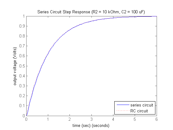
Applying the following MATLAB commands, where the output of our Simulink model from above eo is saved as a time series, will generate the plot shown below.

         s = tf('s');
         R1 = 10;                                          % resistance of resistor in LRC circuit
         R2 = 10000;                                       % resistance of resistor in RC circuit
         Req = 40;                                         % inductor equivalent series resistance (ESR)
         L = 1;                                            % inductance of inductor 
         C1 = 510*10^-6;                                   % capacitance of capacitor in LRC circuit
         C2 = 100*10^-6;                                   % capacitance of capacitor in RC circuit
         ei = 1.53;                                        % battery voltage
         tstep = 1.67;                                     % time step occurred
         G1 = 1/(C1*L*s^2 + C1*(R1+Req)*s + 1);            % LRC circuit transfer function
         G2 = 1/(C2*R2*s+1);                               % RC circuit transfer function
         G = G1*G2;                                        % series transfer function
         [y,t] = step(G*ei,6);                             % model step response with battery voltage scaling
         plot(t,y)
         hold
         plot(eo.Time(100*tstep:100*tstep+599)-tstep+0.01,eo.Data(100*tstep:100*tstep+599),'r:') % experimental
         data
         xlabel('time (sec)')
         ylabel('output voltage (Volts)')
         title('Series Circuit Step Response (R2 = 10 kOhm, C2 = 100 uF)')
         legend('model','experiment','Location','SouthEast')

Examining the above, the predicted and actual responses are quite similar. This seems to indicate that the loading effect was negligible. In general, if the downstream circuit has a significantly higher impedance than the upstream circuit, then the loading effect may be neglected.

Before we investigate the effect of an RC circuit with a smaller impedance, let's first try to understand the response observed for this set of components. One application of an RC circuit like the one employed here is as a low-pass filter. Recalling from Activity 1b, we examined the frequency response of this RC circuit. We saw that this circuit begins to attenuate frequencies above approximately 1 rad/sec. For the given components, the LRC circuit employed above has poles of approximately $-24.8 \pm 36.8j$ (refer to Activity 2a). This means the LRC circuit has a damped natural frequency of 36.8 rad/sec. This is the frequency with which the LRC circuit's response will naturally oscillate. Since 36.8 rad/sec is more than a decade above the RC circuit's break frequency of 1 rad/sec, that means the RC circuit should filter out the oscillation from the LRC circuit. The figure shown below attempts to illustrate this fact. In the figure, one can see that the response of the LRC circuit to a step in input voltage oscillates (has overshoot), but after this signal passes through the RC circuit, the oscillation has been smoothed out.

Another way to interpret the above figure is to recognize that the dynamics of the RC circuit are much slower than the dynamics of the LRC circuit. The "speed" of a system's response is indicated by the size of the real parts of its poles. Since the RC circuit has a pole of -1 and the LRC circuit has poles with real part -24.8, we can think of the LRC circuit as being 25 times "faster" than the RC circuit. This fact is shown in the above figure in that the LRC circuit reaches steady state approximately 25 times sooner than the RC circuit would on its own (recall that settling time $t_s \approx 4/\sigma = 4\tau$ ). In general, the slowest dynamics in a system will dominate the response. Therefore, since the RC circuit is so much slower than the LRC circuit, the RC circuit will dominate the response. Specifically, when the difference in speed (real part of the poles) is greater than a factor of about 5 times, then the fast dynamics can be approximately neglected. This can be observed in the above in that compared to the output of the RC circuit, the output of the LRC circuit looks almost like a step (aside from the overshoot). In fact, if we look at the response of this series circuit compared to the step response of the RC circuit by itself, the outputs are almost indistinguishable. See the figure below for a demonstration of this fact.

In the above, the impedance of the RC circuit was much greater than the LRC circuit, allowing us to treat the two circuits independently (we could neglect the loading effect). Now let's investigate the effect of an RC circuit with smaller impedance. Recall that the resistor in the RC circuit has an impedance of $R_2$ and the and the capacitor has an impedance $1/(sC_2)$ . Therefore, to decrease the impedance of the RC circuit we will reduce $R_2$ and will increase $C_2$ . Specifically, we will try $R_2 = 10\ \Omega$ and $C_2 = 1200\ \mu F$ . Running our experiment with these new components, we generate the following response.

Then using the following code, we can compare the above results to those predicted by our series model.

         s = tf('s');
         R1 = 10;                                          % resistance of resistor in LRC circuit
         R2 = 10;                                          % resistance of resistor in RC circuit
         Req = 40;                                         % inductor equivalent series resistance (ESR)
         L = 1;                                            % inductance of inductor 
         C1 = 510*10^-6;                                   % capacitance of capacitor in LRC circuit
         C2 = 1200*10^-6;                                  % capacitance of capacitor in RC circuit
         ei = 1.53;                                        % battery voltage
         tstep = 1.37;                                     % time step occurred
         G1 = 1/(C1*L*s^2 + C1*(R1+Req)*s + 1);            % LRC circuit transfer function
         G2 = 1/(C2*R2*s+1);                               % RC circuit transfer function
         G = G1*G2;                                        % series transfer function
         [y,t] = step(G*ei,1);                             % model step response with battery voltage scaling
         plot(t,y)
         hold
         plot(eo.Time(100*tstep:100*tstep+99)-tstep+0.01,eo.Data(100*tstep:100*tstep+99),'r:') % experimental
         data
         xlabel('time (sec)')
         ylabel('output voltage (Volts)')
         title('Series Circuit Step Response (R2 = 10 Ohm, C2 = 1200 uF)')
         legend('model','experiment','Location','SouthEast')

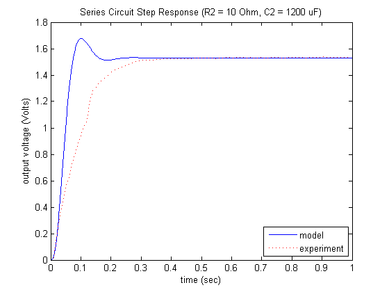
Examination of the above demonstrates that our simplified model does not accurately predict the response observed from our series circuit. It is likely this difference is due to the loading effect which we did not model. In the next section we will investigate this effect in greater detail.

Modeling with loading

In order to address the loading, we will need to re-derive our model for this system to consider the upstream and downstream circuit simultaneously. We will define the current around the first loop to be $i_1$ and around the second loop to be $i_2$ .

Applying Kirchhoff's Voltage Law (the loop law) to the first loop of our circuit, we generate the following equation.

(6) $e_i - R_1 i_1 - L\frac{di_1}{dt} - R_{eq} i_1 - \frac{1}{C_1}\int (i_1 - i_2) \ dt = 0$

Then doing the same for the second loop generates the expression shown below.

(7) $-R_2 i_2 - \frac{1}{C_2}\int i_2 \ dt - \frac{1}{C_1}\int (i_2 - i_1) \ dt = 0$

In order to generate the transfer function model of this circuit, we then need to take the Laplace transform of the two above equations.

(8) $E_i(s) - R_1 I_1(s) - LsI_1(s) - R_{eq}I_1(s) - \frac{1}{C_1s}(I_1(s) - I_2(s)) = 0$

(9) $-R_2 I_2(s) - \frac{1}{C_2s}I_2(s) - \frac{1}{C_1s}(I_2(s) - I_1(s)) = 0$

Next we must perform some algebra to re-arrange the above into the form of a transfer function. In this case, our input is $E_i(s)$ and our output is $E_o(s)$ . Therefore, we must eliminate current $I_1(s)$ and $I_2(s)$ from the above since they are neither inputs nor outputs. We can eliminate and introduce the output using the following relationship, where is the voltage across capacitor $C_2$ .

(10) $E_o(s) = \frac{1}{C_2s}I_2(s)$

Therefore, the two loop equations become the following.

(11) $E_i(s) + \frac{C_2}{C_1}E_o(s) = (R_1 + sL + R_{eq} + \frac{1}{C_1s})I_1(s)$

(12) $(R_2C_2s + 1 + \frac{C_2}{C_1})E_o(s) = \frac{1}{C_1s}I_1(s)$

Solving the two loop equations for $I_1(s)$ and setting equal then eliminates the other current variable.

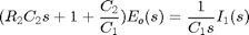
(13) $\frac{E_i(s) + \frac{C_2}{C_1}E_o(s)}{R_1 + sL + R_{eq} + \frac{1}{C_1s}} = \frac{(R_2C_2s + 1 + \frac{C_2}{C_1})E_o(s)}{\frac{1}{C_1s}}$

Performing some algebra, we can generate the resulting transfer function model for this circuit.

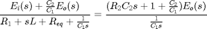
(14) $\Rightarrow G = \frac{E_o(s)}{E_i(s)} = \frac{1}{LR_2C_1C_2s^3 + ((R_1 + R_{eq})R_2C_1C_2 + LC_1C_2)s^2 + ((R_1 + R_{eq})(C_1 + C_2) + R_2C_2)s + 1}$

Comparing to the transfer function $G_{series}$ we derived by considering the LRC and RC portions of the circuit separately, we can see that the downstream circuit does indeed load the upstream circuit.

(15) $G_{series} = \frac{1}{LR_2C_1C_2s^3 + ((R_1 + R_{eq})R_2C_1C_2s + LC_1)s^2 + ((R_1 + R_{eq})C_1 + R_2C_2)s + 1}$

The above models demonstrate our intuition that when the RC circuit is high impedance, the loading effect is negligible. Specifically, when $C_2$ is relatively small and $R_2C_2$ is relatively large, then the true system model $G(s)$ is well approximated by the system model where we modeled the two circuits separately $G_{series}(s)$ .

Executing the code shown below, we can compare our improved model with the observed output.

         s = tf('s');
         R1 = 10;                                          % resistance of resistor in LRC circuit
         R2 = 10;                                          % resistance of resistor in RC circuit
         Req = 40;                                         % inductor equivalent series resistance (ESR)
         L = 1;                                            % inductance of inductor 
         C1 = 510*10^-6;                                   % capacitance of capacitor in LRC circuit
         C2 = 1200*10^-6;                                  % capacitance of capacitor in RC circuit
         ei = 1.53;                                        % battery voltage
         tstep = 1.37;                                     % time step occurred
         G = 1/(s^3*L*R2*C1*C2+s^2*((R2*C1*C2)*(R1+Req)+L*(C1+C2))+s*((C1+C2)*(R1+Req)+R2*C2)+1);
         % improved transfer function
         [y,t] = step(G*ei,1);                             % model step response with battery voltage scaling
         plot(t,y)
         hold
         plot(eo.Time(100*tstep:100*tstep+99)-tstep+0.01,eo.Data(100*tstep:100*tstep+99),'r:') % experimental
         data
         xlabel('time (sec)')
         ylabel('output voltage (Volts)')
         title('Series Circuit Step Response (R2 = 10 Ohm, C2 = 1200 uF)')
         legend('model','experiment','Location','SouthEast')

Examination of the above figure demonstrates that our new model that explicitly addressed the loading agrees with the experimental data to a much greater degree.

Adding an isolating amplifier

If we wish to implement two circuits in series such that the loading effect can be neglected, one option is to employ an Isolating Amplifier between the output of the upstream circuit and the input of the downstream circuit. An isolating amplifier is a non-inverting amplifier with gain equal to one. It is also referred to as a Voltage Follower or a Buffer.

Below is given a schematic of how an operational amplifier can be configured as a buffer between our LRC and RC circuit, where the output of the LRC circuit is connected to the non-inverting input of the operational amplifier. One thing to note is that in order to implement an isolating amplifier, additional power must be supplied to the operational amplifier. Referring to our earlier observations of the step response for the LRC circuit, we need our isolating amplifier to follow a voltage input approaching 2 Volts for a 1.5 Volt input. This corresponds to a single alkaline battery source and an underdamped response that overshoots the input voltage. Since no operational amplifier can supply the theoretical maximum voltage, we should employ a positive and negative supply of at least +3 Volts and -3 Volts relative to ground, respectively. This supply can be provided via a DC power supply, or from additional batteries. For example, two 9-Volt batteries (one for the positive supply and one for the negative supply) can be employed, or multiple AA batteries can be employed in series. If an insufficient power supply is provided to the operational amplifier, it will begin to behave nonlinearly at higher voltage inputs. In other words, it will begin to saturate.

For our experiment, we will employ a relatively inexpensive, general purpose operational amplifier, the LM741, whose datasheet can be found here. The numbers indicated on the operational amplifier in the above figure correspond to the pin-outs of this model. Such an operational amplifier will introduce a bias that can be removed by adjusting a trimming potentiometer between the offset null pins 1 and 5. Since the bias is relatively small (< 6 mV) we will neglect to do this.

Setting up the circuit with isolating amplifier as described, we can re-run our Simulink program (making sure to first discharge both capacitors). Employing the same LRC components that we have been, along with the RC circuit with components $R_2 = 10\ \Omega$ and $C_2 = 1200\ \mu F$ , generates the following response.

Executing the following commands in MATLAB then allows us to compare the response of the circuit to the model $G_{series}(s)$ that we derived by neglecting the effect of loading.

         s = tf('s');
         R1 = 10;                                          % resistance of resistor in LRC circuit
         R2 = 10;                                          % resistance of resistor in RC circuit
         Req = 40;                                         % inductor equivalent series resistance (ESR)
         L = 1;                                            % inductance of inductor 
         C1 = 510*10^-6;                                   % capacitance of capacitor in LRC circuit
         C2 = 1200*10^-6;                                  % capacitance of capacitor in RC circuit
         ei = 1.54;                                        % battery voltage
         tstep = 1.63;                                     % time step occurred
         G1 = 1/(C1*L*s^2 + C1*(R1+Req)*s + 1);            % LRC circuit transfer function
         G2 = 1/(C2*R2*s+1);                               % RC circuit transfer function
         G = G1*G2;                                        % series transfer function
         [y,t] = step(G*ei,1);                             % model step response with battery voltage scaling
         plot(t,y)
         hold
         plot(eo.Time(100*tstep:100*tstep+99)-tstep+0.01,eo.Data(100*tstep:100*tstep+99),'r:') % experimental
         data
         xlabel('time (sec)')
         ylabel('output voltage (Volts)')
         title('Series Circuit Step Response with Isolating Amplifier')
         legend('model','experiment','Location','SouthEast')

As expected, inspection of the above shows relatively good (though not perfect) agreement between the data and the model. The addition of the isolating amplifier allows us to mostly neglect the loading effect we had observed earlier. Much of the difference between the model and the data can be attributed to mismatch between the actual and assumed component values, and to the unmodeled effects of the measurement channel.

If we consider the RC circuit in this example to be a low-pass filter, there are alternative implementations of low-pass filters that also allow us to neglect this loading effect. Specifically, the implementation of a low-pass filter employed here is a passive implementation that can cause the input signal to be attenuated. Alternative active implementations often employ operational amplifiers in much the same way the isolating amplifier we implemented here does.