Suspension: Simscape Modeling

Physical setup

In this section, we show how to build the suspension model using Simscape. The blocks in Simscape represent actual physical components, enabling the user to create complex multi-domain models without deriving and implementing mathematical equations from first principles.

Specifically, we will replicate the Simulink model developed in the Suspension: Simulink Modeling page using Simscape and will additionally implement the closed-loop control described in Suspension: Simulink Controller Design. The suspension representation is repeated below.

Recall, the system parameters are as follows.

(m1)    body mass                                2500 kg

(m2)    suspension mass                          320 kg

(k1)    spring constant of suspension system     80,000 N/m

(k2)    spring constant of wheel and tire        500,000 N/m

(b1)    damping constant of suspension system    350 N.s/m

(b2)    damping constant of wheel and tire       15,020 N.s/m

(u)     control force = force from the controller we are going to design

Design requirements

The design requirements are also the same as previously defined. We aim to design a feedback controller so that the output (X1-X2) has an overshoot less than 5% and a settling time shorter than 5 seconds.

Open a new model

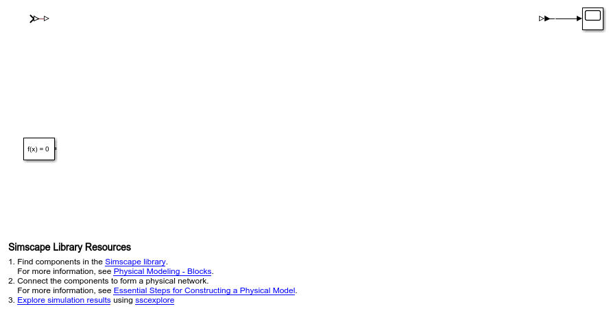
Open a new Simscape model by typing ssc_new in the MATLAB command window. A new model opens up with a few commonly used blocks already in the model. Furthermore, you will need to define the associated suspension model parameters in the MATLAB workspace. This can be accomplished by running the file suspension_parameters.m which can be downloaded by right-clicking and selecting Save link as ....

Assemble system to represent tire and road inputs

Below are the blocks to add. Tips:

Use Quick Insert to add the blocks. Click in the diagram and type the name of the block (use the letters in bold below). A list of blocks will appear and you can select the block you want from the list.
After the block is entered, a prompt will appear for you to enter the parameter. Enter the variable names as shown below.
To rotate a block or flip blocks, right-click on the block and select the desired option from the Rotate & Flip menu.
To show the parameter below the block name, see Set Block Annotation Properties in the Simulink documentation

Mechanical Translational Reference
Ideal Translational Velocity Source
Translational Spring (Spring rate = "k2")
Translational Damper (Damping coefficient = "b2")
Mass (Mass = "m2")
Pulse Generator (Amplitude = "1")

For the Pulse Generator block, double-click on the block and set Period to "100" and Pulse Width to "0.1".

Connect the blocks as shown below. Connect the output of the Pulse Generator to the Simulink-PS Converter block that is already in the diagram in the upper left corner (two triangles with a Simulink input), and connect the output of that block to the Ideal Translational Velocity Source.

You can give the blocks meaningful names by clicking on the blocks, then clicking on the name and editing it.

Sense key values and simulate

The following steps will allow the display of the simulation results on the Scope.

Connect the R port of the Ideal Translational Motion Sensor as shown below.
Make a copy of the Mechanical Translational Reference block to connect to the C port of the sensor.
Connect the v port of the sensor to the PS-Simulink converter already in the diagram (white trangle and black triangle which is connected to the Scope)
Make a copy of the PS-Simulink converter, and connect the p port to the Scope via the converter block as shown below.

Before running the simulation, set the maximum step size to 1e-2 using the following steps.

Type CTRL-E to open the Configuration Parameters dialog
Click on the Solver Pane
Expand the Solver details section
Set Max step size to "1e-2"

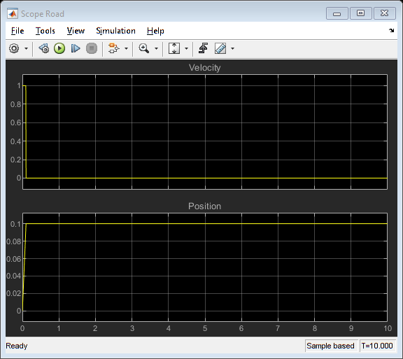
Then run the simulation (CTRL-T or press the green arrow run button). You will see the response of the bus (one wheel) as it encounters a 0.1 m bump as shown in the Scope.

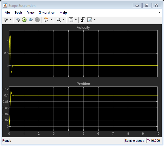
Define vehicle system

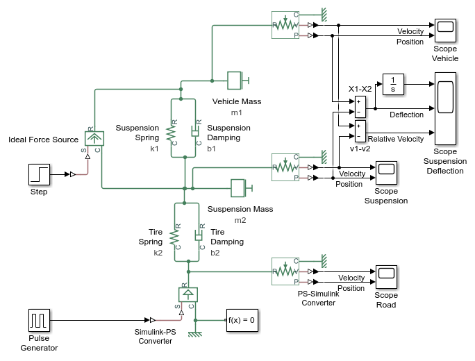
You can copy and paste the spring, damper, mass, and sensor blocks to model more of the vehicle with a second mass-spring-damper. Click and drag to select the blocks, then right-click on one of the selected blocks and drag to copy them.

You will need to set the parameters to m1, b1, and k1, and we recommend giving the blocks meaningful names. The resulting model is shown below.

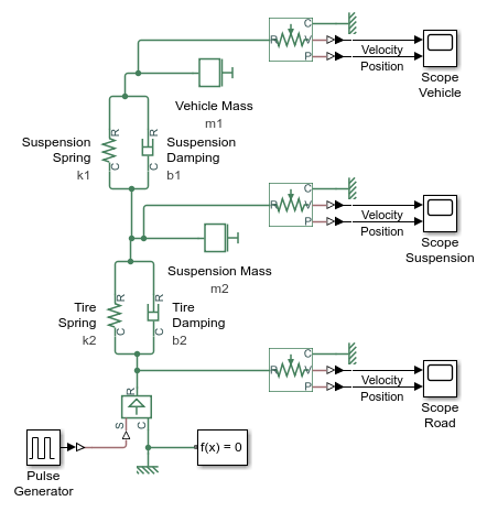
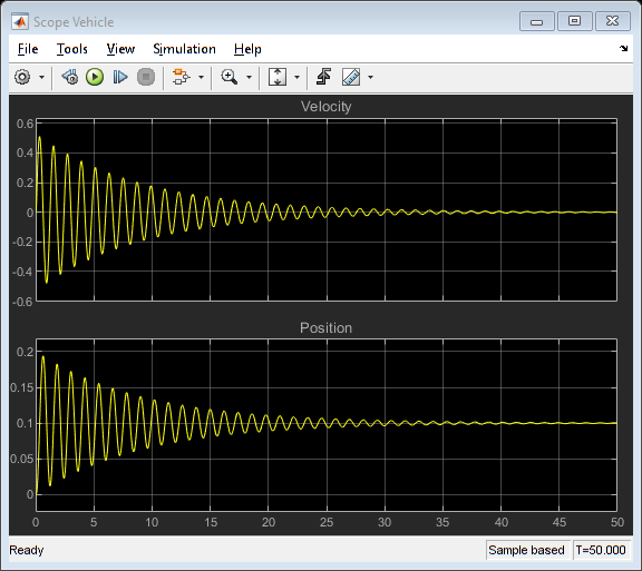
Then run the simulation (type CTRL-T). You will see the vehicle body oscillates for a long time. Set the stop time to 50 seconds to see for how long it oscillates.

Define control input and measure additional states

Now we add an Ideal Force Source as shown below so that our control system can apply a force to quickly damp out the oscillations from the bump. To perform an open-loop test of the actuator, add a Step block and set the Step Time to "0". Turn off the road input by setting the Amplitude of the Pulse Generator to "0".

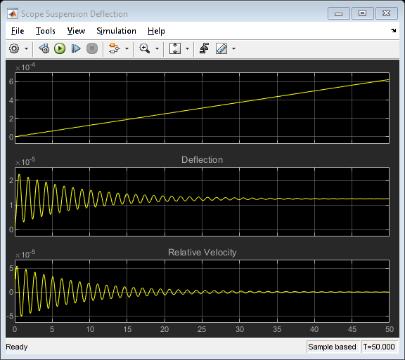
To measure the suspension deflection, add two Subtract blocks to calculate the difference between the relative positions and velocities of the vehicle and the suspension. Then add an integrator to integrate the difference in relative motion of the vehicle and suspension.

Running the simulation, the resulting suspension response on the Suspension Deflection Scope should appear as follows.

Create closed-loop control

For clarity, place the suspension model in a subsystem following the steps below.

Replace the Scope blocks with Out1 blocks and the two inputs with In1 blocks
Click and drag to select all blocks except the Step, Pulse Generator, Scope Vehicle, and Scope Suspension Deflection blocks
Type CTRL-G (or right-click and choose) to create the subsystem
Resize the subsystem so that all ports can be seen

The outputs of this system are the states that will be used by the controller (see the Suspension: State-Space Controller Design page for details). We wish to label them and order them the same as used for the control design steps. Rename and re-order the outputs as shown in the screenshot below.

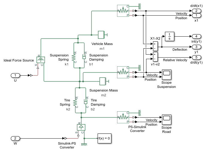
Back at the top level, delete the output connections and connect the subsystem outputs to a Mux block as shown below. When you add the Mux block, you can set the parameter Number of inputs to "5". The output of the Mux block is the state vector that will be used by the controller.

To use the control gains, add a Gain block and set parameter Gain to "K". Double-click on the block and set the Multiplication parameter to "Matrix (K*u)". Connect the output of the Mux block to the input of the Gain block. The output of this block will be subtracted from the command signal to generate the actuator command.

Add a Subtract block, and connect the Gain and Step blocks as shown below. Connect the output of the subtract block to the input that connects to the Ideal Force Source in the suspension subsystem.

Before running the simulation, set the inputs to model the case of the bus going over a bump. Also note that the feedback gain matrix K is defined in the file suspension_parameters.m, where K = [ 0 2.3E6 5E8 0 8E6 ].

In the Step block, set the Final value parameter to "0".
In the Pulse Generator block, set the Amplitude to "1".

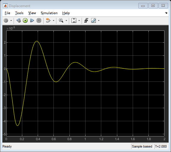
Then run the simulation (CTRL-T or press the green arrow run button). The Scope shows that the displacement of the vehicle is much smaller than before due to the control system. You can set the stop time to 2 seconds to see the oscillations in more detail.

You can download the final Simscape model created here by right-clicking here and then selecting Save link as ....